Jedi Simon Linkshaa Solution
Jedi
Simon Foundation
Resonant Vibration Department Research - Cymatics Research -
Approccio Sinergico Integrato: Linkshaa Science
per risolvere quello che una sola scienza non puo',
al servizio della vita. Multivariable Earthquake precursors.
Si applichi nel caso di vita o di morte il Diritto condiviso della
conoscenza, al servizio dell'uminatià.
Nel nome della conoscenza, della consapevolezza nell'interesse della comunità.
L’Aquila 30 Novembre 2006 Cronistoria dell’attività di Ricerca
della S C S sui “Precursori di eventi sismici”.Anni 2000-2001
Un piccolo gruppo di Fisici e Tecnici che lavorano presso i Laboratori Nazionali
del Gran Sasso
(CNR-INFN) decidono, per comune interesse e curiosità scientifica, di iniziare
una ricerca basata su
un nuovo metodo di misura delle emissioni di 222Radon.
Questa ricerca e’ interamente privata e viene fatta con strumentazione
riadattata e installata in uno
scantinato di una civile abitazione alla periferia dell’Aquila.
Le persone coinvolte sono:
Sig. Gioacchino Giuliani – CTER - IFSI - LNGS
Sig. Roberto Giuliani – Tecnico Informatico INFN – LNGS
Prof. Victor Alekseenko - Ricercatore del Baksan Neutrino Astronomy (Russia)
L’interesse per questa ricerca, era rappresentato dalla possibilità di poter
determinare con certezza, se
le variazioni di concentrazione di Radon emesse dalla crosta terrestre, in
prossimità di un terremoto,
avvenissero prima dell’evento, durante o dopo.
Va segnalato che ricerche su emissioni di 222Radon mirate alla possibilità di
osservare Precursori
sismici, sono state effettuate nel corso degli ultimi 40 anni, da ricercatori e
università di tutto il
mondo, ma senza ottenere mai risultati significativi.
A tutt’oggi ricerche di questo tipo sono ancora in corso.
Anni 2001-2002
Il primo periodo di lavoro, è stato speso per realizzare un sismografo a pendolo
verticale.
Essenzialmente il sismografo avrebbe fornito informazioni sulla dinamicità
nell’area di sensibilità del
rivelatore di Radon, e tracciare una mappa sismogenetica locale, per ottenere un
rapporto di
correlazione tra flusso medio di Radon e l’attività dinamica prodotta dagli
eventi sismici osservati.
L’importanza di un sismografo per le correlazioni delle variazioni di
concentrazione di Radon ed
eventi sismici, risulta essenziale per la determinazione della sismogeneticità
della zona e la media
statistica di eventi per anno, per stagione, per mese.
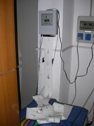
L’immagine a sinistra mostra il sismografo a pendolo verticale.
Esso è stato posizionato a circa tre metri di distanza dal prototipo rivelatore
di Radon. Entrambi i sensori, sono tutt’ora localizzati in una stanza interrata
a circa tre metri di profondità, in assenza di ventilazione.
Il secondo periodo di attività è stato dedicato alla realizzazione di diversi
tipi di contatori, per
ricercare un metodo ed una tecnica attendibili.
E’ naturale, credo, che dovendo trovare correlazioni tra un elemento ed un
fenomeno tra loro
associabili, si puntualizzi lo studio o sull’elemento o sul fenomeno.
Parve quindi naturale, realizzare degli strumenti artigianali, per il
rilevamento di particelle alfa
prodotte dal decadimento del Radon attraverso delle semplici camere a
ionizzazione o tubi
proporzionali.
Ricordiamo, per i meno informati, alcuni elementi caratteristici del Radon.
Esso è un elemento mobile, radioattivo e chimicamente inerte, questa doppia
proprietà, di essere
elemento estremamente mobile e chimicamente non reattivo, gli danno
l’appellativo di elemento
nobile.
In natura si trovano tre isotopi del Radon, il 222Rn prodotto dall’ 238U, il
220Rn prodotto dal 232Th ed il
219Rn prodotto dal 235U.
Dalle diverse catene di decadimento radioattivo, 238U, 232Th e 235U, tutti gli
isotopi del Radon vengono
prodotti per emissione di particella alfa dall’elemento 226Radio.
Sono state così realizzati due tipi di contatori, uno a camera di ionizzazione
ed uno a tubi, così come
mostrano le immagini seguenti.
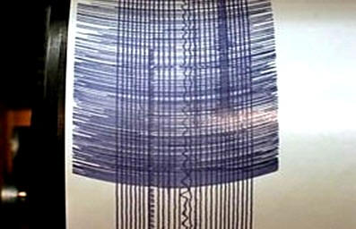
L’immagine a destra mostra la sezione digitale del sismografo. Essa è costituita
dal sistema di taratura, dal datario e dalla
stampante termica per i sismogrammi. E’ tra l’altro prevista la possibilità di
inviare il segnale sismico direttamente su un Pc,
che permette di avere un allarme sonoro in coincidenza dell’evento sismico.
L’ immagine a sinistra mostra 2 camere a ionizzazione, costituita da due piastre
contrapposte, (Catodo), attraversate nella parte centrale e lungo la
diagonale da un cavo di circa 40 μm (Anodo) sul quale viene applicata una
tensione di circa 1700 V.
Il campo elettrico prodotto all’interno della camera, permette di osservare la
cascata elettronica prodotta dal passaggio degli ioni di Radon e dei gas
presenti
nell’ambiente.
Il secondo periodo di attività è stato dedicato alla realizzazione di diversi
tipi di contatori, per
ricercare un metodo ed una tecnica attendibili.
E’ naturale, credo, che dovendo trovare correlazioni tra un elemento ed un
fenomeno tra loro
associabili, si puntualizzi lo studio o sull’elemento o sul fenomeno.
Parve quindi naturale, realizzare degli strumenti artigianali, per il
rilevamento di particelle alfa
prodotte dal decadimento del Radon attraverso delle semplici camere a
ionizzazione o tubi
proporzionali.
Ricordiamo, per i meno informati, alcuni elementi caratteristici del Radon.
Esso è un elemento mobile, radioattivo e chimicamente inerte, questa doppia
proprietà, di essere
elemento estremamente mobile e chimicamente non reattivo, gli danno
l’appellativo di elemento
nobile.
In natura si trovano tre isotopi del Radon, il 222Rn prodotto dall’ 238U, il
220Rn prodotto dal 232Th ed il
219Rn prodotto dal 235U.
Dalle diverse catene di decadimento radioattivo, 238U, 232Th e 235U, tutti gli
isotopi del Radon vengono
prodotti per emissione di particella alfa dall’elemento 226Radio.
Sono state così realizzati due tipi di contatori, uno a camera di ionizzazione
ed uno a tubi, così come
mostrano le immagini seguenti.
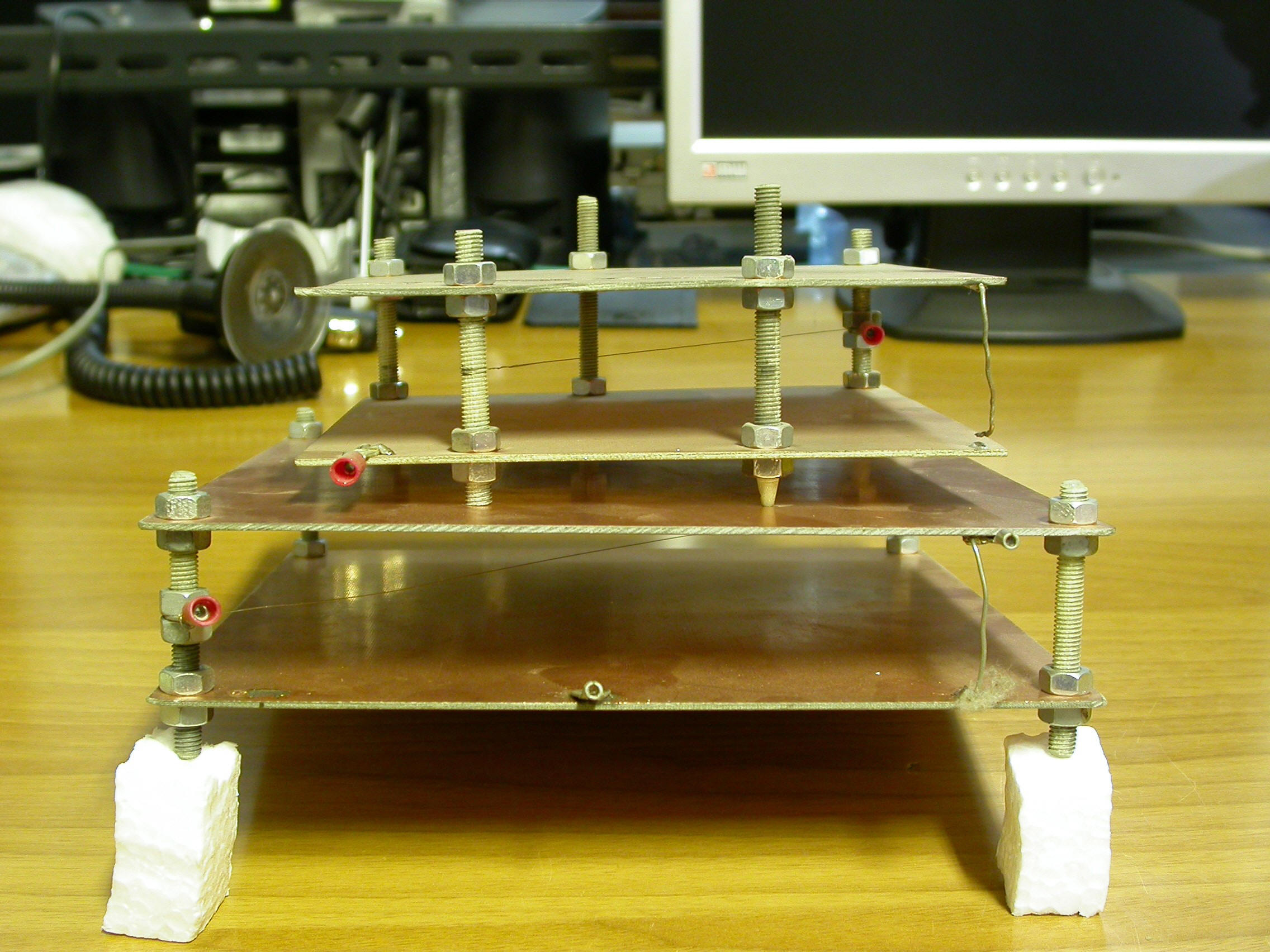
L’ immagine in alto mostra 2 camere a ionizzazione, costituita da due piastre
contrapposte, (Catodo), attraversate nella parte centrale e lungo la
diagonale da un cavo di circa 40 μm (Anodo) sul quale viene applicata una
tensione di circa 1700 V.
Il campo elettrico prodotto all’interno della camera, permette di osservare la
cascata elettronica prodotta
dal passaggio degli ioni di Radon e dei gas presenti nell’ambiente.
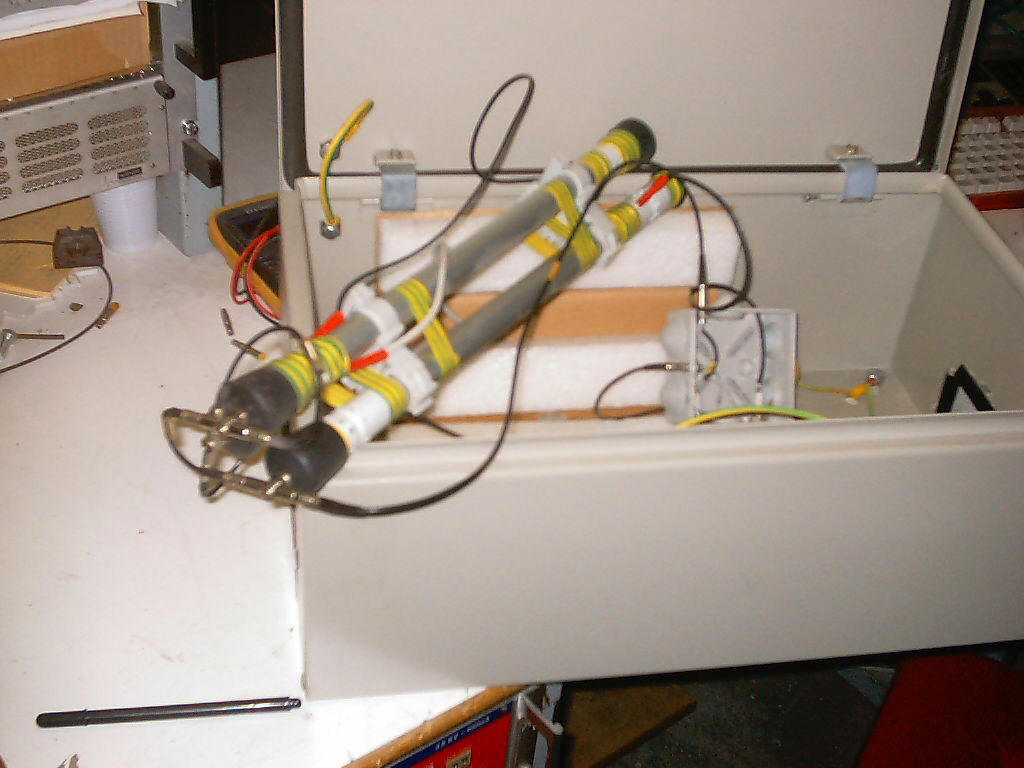
L’immagine in basso mostra invece un rivelatore costituita da 3 tubi, il cui
funzionamento si basa sullo
stesso principio delle camere precedenti. Anche in questo caso l’interno del
cilindro è attraversato da un cavo di 40 μm,
sul quale è applicata una tensione continua negativa, pari a circa 1400 – 1600
V.
La figura in alto mostra lo schema elettrico utilizzato sia per le camere a
ionizzazione che per i tubi.
Il sistema sopra descritto, dopo un paio di mesi di test, si è rivelato poco
pratico ed anche piuttosto
impreciso per le informazioni che volevamo ottenere.
Le camere a ionizzazione non hanno una buona velocità di risposta, quando il
flusso del gas risulta
piuttosto elevato, per cui si incontrano difficoltà sostanziali nell’utilizzare
questi strumenti come
rivelatori di impulsi singoli.
Nel periodo Gennaio, Febbraio 2001, risultò subito evidente che bisognava
cambiare metodo di
ricerca, la strada che si stava perseguendo, avrebbe dato informazioni
esclusivamente sulla
concentrazione relativa del Radon nell’ambiente.
La stessa risposta si sarebbe potuta ottenere acquistando un normale Radometro,
ma l’incidenza del
costo, per un discreto strumento, e le risposte scientifiche che avremmo
ottenuto, sarebbero state le
stesse acquisite fino ad oggi dalla scienza ufficiale; perciò si decise di
seguire una strategia di ricerca
diversa da quella tradizionale.
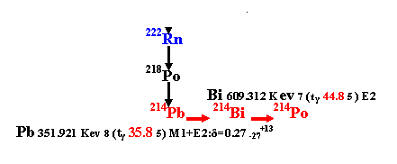
Il grafico in basso, mostra la catena di decadimento dell’ 238Uranio ed è da
questa catena che si è
intuito, su quale ramo di decadimento del Radon si dovesse focalizzare
l’attenzione per realizzare un
nuovo rivelatore che permettesse misure correlabili con eventi sismici.
Attraverso un’attenta osservazione della catena di decadimento del 222Rn, in
modo particolare nella
fase in cui vengono prodotti gli isotopi 214Pb, 214Bi e 214Po, si osserva che
questi elementi, a differenza
degli altri, anziché decadere con processo alfa, decadono con processo beta, con
emissione di fotoni
gamma.
(L’immagine seguente mostra la sezione della catena, nella fase di decadimento
beta)
Disponendo quindi di alcuni Fotomoltiplicatori e di scintillatore plastico, è
stato realizzato un primo
prototipo che ci avrebbe permesso di contare flash di particelle gamma prodotte
dal decadimento beta
del 214Pb e del 214Bi.
La rivelazione di questi elementi, con questo metodo, ci avrebbe permesso di
rilevare impulsi singoli
con buona precisione; inoltre essendo essi diretti isotopi del Radon, il valore
della loro variazione di
concentrazione, equivaleva alla variazione di concentrazione del Radon emesso
dalla crosta terrestre.
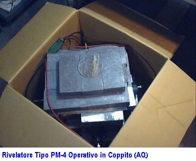
Nasce così il primo prototipo di particelle gamma, costituito da 4
fotomoltiplicatori ed uno
scintillatore plastico.
Esso viene posto in acquisizione in uno scantinato ad una profondità di tre
metri dalla superficie
stradale, nella zona di Coppito (AQ), nel mese di Maggio 2002.
L’immagine a sinistra mostra il primo rivelatore chiamato PM4, durante la
fase di preparazione e prima di entrare in
funzione, presso la stazione di rilevamento di Coppito (AQ)
Il grafico a destra rappresenta il primo counting rate ottenuto dopo i primi
periodi di acquisizione del rivelatore
PM4 di Coppito (AQ). Sulle ascisse sono riportate le ore relative ai giorni di
presa dati, dal 27/06/02 al 01/07/02
Sulle ordinate è riportato il numero degli eventi ogni 7200 secondi, (Counting
rate).
Già dalle prime settimane di presa dati, i risultati apparvero più che
soddisfacenti.
Si era centrato l’obbiettivo! Per la prima volta, si osservava un segnale
continuo che rappresentava la
variazione di concentrazione di Radon, ottenuta dall’osservazione di suoi
diretti figli di decadimento:
gli isotopi di 214Pb e 214Bi.
Dopo alcuni mesi, dedicati alla taratura dell’elettronica ed allo studio del
segnale prodotto, vengono
ottenute le prime correlazioni tra variazione di concentrazione di Radon ed
eventi sismici.
Nel periodo Luglio-Ottobre 2002, i dati osservati vengono analizzati con il
metodo della Varianza.
Ogni settimana, veniva controllata la media di flusso del Radon, cercando
anomalie nel counting rate
acquisito; contemporaneamente il sismografo monitorava l’attività sismica
relativa a piccoli eventi
registrati in prossimità delle coordinate del rivelatore PM4, (Lat. +42° 21’N,
Long. +13° 20’E).
L’immagine a sinistra mostra il primo rivelatore chiamato PM4, durante la fase
di preparazione
e prima di entrare in funzione, presso la stazione di rilevamento di Coppito
(AQ)
Il grafico a destra rappresenta il primo counting rate ottenuto dopo i primi
periodi di
acquisizione del rivelatore PM4 di Coppito (AQ).
Sulle ascisse sono riportate le ore relative ai giorni di presa dati, dal
27/06/02 al 01/07/02
Sulle ordinate è riportato il numero degli eventi ogni 7200 secondi, (Counting
rate).
Giorno Lat. Long. Area Magnitudo
03/08/2002 42°.6 13°.0 C. Italia M 3.2
06/09/2002 41°.9 12°.5 S. Italia M 4.5
07/09/2002 41°.6 15°.8 S. Italia M 2.7
09/09/2002 42°.4 11°.8 C. Italia M 4.5
24/09/2002 41°.7 13°.3 S. Italia M 2.5
06/10/2002 39°.6 12°.4 Tirreno M 3.2
19/10/2002 40°.7 12°.7 Tirreno M 2.9
23/10/2002 42°.7 17°.3 Adriatico M 4.0
Ii- counting rate di due ore
La tabella di seguito mostra i primi allarmi prodotti dall’analisi della media
del flusso di Radon
osservato e correlato con gli eventi sismici, registrati e dal nostro sismografo
e dalla Sala sismica
centrale dell’INGV di Roma.(www.ingv.it)
PRIME CORRELAZIONI TRA VARIAZIONI DI
CONCENTRAZIONE DI RADON ED EVENTI SISMICI
DATA LAT. LOMG. ORA Previsto MAG.
Ev.
03/08/2002 42°.6 13°.0 19.21 02/08/2002 M. 2.7
06/09/2002 41°.9 12°.5 13.45.00 05/09/2002 M. 4.5
07/09/2002 41°.6 15°.8 7.38.16 06/09/2002 M. 2.7
09/09/2002 42°.4 11°.8 2.53.46 08/09/2002 M. 4.5
24/09/2002 41°.7 13°.3 15.22.09 23/09/2002 M. 2.5
06/10/2002 39°.6 12°.4 1.22.41 05/10/2002 M. 3.2
19/10/2002 40°.7 12°.7 16.02.51 18/10/2002 M. 2.9
23/10/2002 42°.7 17°.3 11.01.25 22/10/2002 M. 4.0
29/10/2002 serie eventi S. Giuliano 31/10/02
30/10/2002 serie eventi S. Giuliano 01/11/02
43°.6 12°.8 11.32 25/03/2003
26/03/2003 19.01 25/03/2003 M. 2.5
30/03/2003 41°.6 14°.7 16.42 29/03/2003 M. 3.3
11/04/2004 42°.30 13°.40 11.04 10/04/2003 M. 2.4
In questo stesso periodo era stata presentata alla Regione Abruzzo e Protezione
Civile Abruzzo, una
richiesta di finanziamento per la nostra ricerca, nella speranza di poter
ammortizzare le spese del
nostro progetto, che seppur condotto in maniera artigianale, incideva
pesantemente sul bilancio
famigliare.
In cambio del finanziamento promesso, la Protezione Civile dell’Aquila, avrebbe
ricevuto dalla sala
sismica della S.C.S., gli allarmi > del 3° Richter, previsti il giorno prima
dell’evento.
Per motivi che qui non stiamo a sottolineare, la S.C.S. non ha mai ricevuto
nessun genere di aiuto.
La tabella in alto mostra gran parte degli eventi allarmati nel periodo Agosto –
Ottobre 2002 alla
Protezione Civile di L’Aquila.
In particolare, le date segnate in rosso nella tabella, mostrano gli allarmi
trasmessi, all’allora
Assessore Regionale ai Lavori Pubblici, con delega per la Protezione Civile, Dr.
Giorgio De Matteis.
Il 20 Dicembre 2002 viene depositata domanda di brevetto sul sistema di
“Precursore di eventi
sismici”
Anno 2003
Sulle ali dell’euforia, il gruppo di ricerca della S.C.S., Roberto Giuliani,
Victor Alekseenko e
Giampaolo Giuliani, per i risultati ottenuti sulle correlazioni Radon -
terremoti e per l’individuazione
del segnale chiamato precursore sismico, decise di incrementare lo sforzo della
ricerca in corso.
Il gruppo era convinto che la scoperta del sistema per rilevare allarmi sismici
da 6 a 24 ore di anticipo
sull’evento, sarebbe stata apprezzata sia nell’ambiente scientifico italiano,
che negli ambienti della
Protezione Civile nazionale.
Confortati dalla certezza, fu deciso di costruire un secondo rivelatore da
posizionare ad una certa
distanza da quello in funzione a Coppito (AQ).
Con l’elettronica e la meccanica ancora disponibile, si dette quindi inizio alla
realizzazione di un
secondo detector, con caratteristiche identiche al primo.
Per questo secondo rivelatore furono utilizzati 2 Fotomoltiplicatori anziché 4
come il precedente.
Questa scelta avrebbe permesso di verificare la riproducibilità del sistema,
l’efficienza, la sensibilità e
l’eventuale correlazione con siti tra loro distanti e diversi.
Bisognava nello stesso tempo incrementare le analisi sui dati forniti dal PM4.
Il dr. V. Alekseenko propose un algoritmo sulla Varianza delle 24 ore del 222Rn,
per mezzo del quale
sarebbero state effettuate correlazioni con le variazioni di concentrazione di
Radon ed un maggior
approfondimento sui diversi fenomeni, quale ad esempio le armoniche, osservate
nel continuo dei dati
rilevati.
Il Sig, G. Giuliani propose un algoritmo sulla media di flusso del 222Rn in
ambiente chiuso e senza
ventilazione, rilevato ogni 2 ore.
Questo algoritmo sarebbe stato applicato al programma automatico di allarmi
sismici sulla rete
internet, con dei messaggi via e-mail.
Formula dell’algoritmo applicato:
| CI – CI+n | > 3 < C > n = 1,…..,12
Dove: < C > = å12
1
Ci /12
Il Sig. R. Giuliani avrebbe organizzato invece un software per il controllo dei
dati acquisiti, adattabile
ad un diverso numero di sistemi tra loro interallacciati e posti sulla rete
internet, per ottenere in tempo
reale preallarmi ed allarmi attraverso le soglie dei precursori sismici connessi
in modo nodale.
Esempio di allarme sismico del 29 dicembre 2005, via e-mail e relativo al sisma
del 30 dicembre
2005 Alta_Val_Tiberina delle ore 10:37U.T. pari a 2,5M:
pm4
ALLARME
Massimo: 29/12/2005 02:00:00 150117
Minimo: 29/12/2005 16:00:00 146780
Differenza: 3337
Arco Tangente: -1,5686986373335159
La necessità di un secondo rivelatore, posto ad una certa distanza dal primo,
avrebbe definitivamente
risposto ai diversi quesiti che assillavano un po’ tutti.
Fino ad allora non si aveva notizia nell’ambiente scientifico, di osservazioni
effettuate sull’emissione
di Radon dalla crosta terrestre, controllata on-line, in tempo reale e da
diversi siti di osservazione.
Gli interrogativi che chiedevano risposte erano:
- Quale andamento dei flussi sarebbe stato osservato dai rivelatori in siti
diversi?
- Quale andamento avrebbero avuto i flussi monitorati, in prossimità di eventi
sismici, rilevati
dai diversi detectors?
- Il flusso e l’andamento del Radon misurato dipendeva anche dalla natura del
terreno dove
venivano situati i rivelatori?
Naturalmente l’interrogativo più importante era costituito dalla necessità di
sapere se due o tre
rivelatori potessero correlarsi tra loro e fornire, con una certa precisione,
epicentro, grado sismico ed
ora dell’evento.
Con un solo rivelatore purtroppo, non era possibile dare una stima
sull’epicentro dell’eventuale sisma
allarmato, se non nel raggio d’azione del rivelatore; mentre era possibile avere
una stima del grado
magnitudo con un errore di circa 0.5°-0.6° di Grado.
Verso Maggio-Giugno 2003, il secondo rivelatore con 2 Fotomoltiplicatori, era
pronto per entrare in
funzione.
Per un periodo di qualche mese, sarebbe stato tarato, al fianco del fratello
chiamato PM4.
Pur lavorando nel campo della ricerca dei precursori sismici, con molta
discrezione ed avendo avuto
relazioni solo con dirigenti della Protezione Civile dell’epoca, fummo
contattati nei mesi Giugno -
Luglio 2003 dall’imprenditore Vincenzo Passarelli.
L’imprenditore si disse interessato alla richiesta di brevetto da noi presentata
in Italia, sul metodo e
tecnica per la rivelazione dei precursori sismici, garantendo la possibilità di
commercializzare
all’estero i nostri rivelatori.
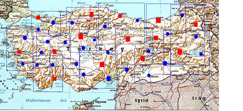
Si giunse ad un accordo definitivo, che prevedeva la realizzazione di due reti
di monitoraggio anti
sismiche, una in Algeria ed una in Turchia, finanziate dai due governi.
Vincenzo Passatelli avrebbe finanziato un test ufficiale da effettuarsi a Reggio
Calabria, sotto l’egida
di un gruppo di Geofisica dell’Università di quella città.
Purtroppo la trattativa si interruppe proprio il giorno della firma per
l’accordo, presso l’ufficio del
legale preposto alla stesura del contratto.
Nel mese di Ottobre 2003, la Caen S.p.a. di Marcello Givoletti ci propose di
subentrare al posto
dell’imprenditore Passatelli.
La Caen rappresenta a tutt’oggi la più importante società italiana per la
produzione di apparecchiature
elettroniche per la fisica nucleare.
La possibilità di essere sostenuti da una così importante società, ci spinse ad
accettare l’offerta del
Presidente Marcello Givoletti.
Data la delicatezza dell’argomento e pur con tutta la “prudenza” necessaria,
d’accordo con Marcello
Givoletti (Caen), sentimmo il dovere di parlare della scoperta con qualche
Istituzione Scientifica.
Il problema era: “cosa fare dei dati che erano stati rilevato” e soprattutto
“cosa sarebbe stato giusto
ancora fare” per tentare di dare, se possibile, una risposta scientifica e
rigorosa sull’argomento.
Più in particolare si pensava di :
- Aprire una o più collaborazioni con Istituzioni o Università?
- Collaborare con qualche Istituto per migliorare l’efficienza del rivelatore di
particelle finora usato?
- Creare una rete di almeno 10-15 sistemi di misura distanti fra loro circa 50
Km col fine di
interpolare le misure di ogni rivelatore (per ottenere una maggiore accuratezza
sulla stima
dell’epicentro) come dimostrano i dati fino ad ora analizzati?
- Studiare un sistema di calibrazione per ogni singolo sistema in funzione della
diversa struttura
geologica del terreno di misura.
- Integrare le misure con altre informazioni (campo elettrico e magnetico
terrestre ??)
- Reperite risorse umane e finanziarie per portare avanti un simile programma
(spese vive valutate
intorno a 500 K€).
Nella seconda metà del 2003 entrammo in contatto con il Sen. Zamberletti,
presidente dell’ISPRO
(www.ispro.it) e notoriamente da sempre coinvolto col fenomeno Terremoti.
Il Sen. Zamberletti si dichiarò molto interessato alla scoperta ed organizzò a
Roma presso i locali
dell’ISPRO, una riunione allargata a una decina di persone interessate
all’argomento fra le quali
citiamo il Prof. Enzo Boschi (Presidente INGV), il Dott.Galanti, Direttore
Servizio Sismico
nazionale, il Gen. Mollicone (Aeronautica Militare), ecc….
Gioacchino Giuliani espose nella circostanza quanto era stato fatto fino a quel
momento,
sottolineando, che tutte le spese erano state sostenute da un auto finanziamento
famigliare.
Espose inoltre, quanto scientificamente fosse stato svolto fino ad allora ,
senza alcuna pretesa, propose
inoltre se poteva essere presa in considerazione la formazione di un gruppo di
lavoro congiunto per
verificare e ampliare il programma di ricerca.
Le reazioni dei singoli partecipanti sono state molto diverse fra loro (in
particolare quella del Prof.
Boschi e’ stata a dir poco “scortese”) , ma complessivamente la riunione non ha
portato a nessuna
conclusione positiva. Va segnalato che nessuno allora (e fino a tutt’oggi) ha
trovato errori o inesattezze sulle misure
effettuate! Al fine di dimostrare ufficialmente che i nostri dati erano
attendibili, fu accettata la proposta dell’On.
Zamberletti, di sottoporre il sistema ad un test di funzionamento. Il Sistema
avrebbe inviato dal 20 Gennaio 2003
all’8 Gennaio 2004, gli “allarmi e preallarmi segnalati” come sismi.
Gli allarmi sarebbero dovuti pervenire un “notaio” di Viareggio, (Al fine di
certificarne la data e l’ora
certa), alla Caen S.p.a. ed alla ISPRO dell’On. Zamberletti.
Gli allarmi e preallarmi spediti, hanno anticipavano gli eventi sismici, con un
intervallo di tempo
variabile dalle 6 e le 24ore. L’operazione riuscì perfettamente.
Nell’incontro successivo effettuato alla ISPRO, il Sen. Zamberletti avanzò
l’ipotesi che un
programma di ricerca congiunto, sarebbe stato finanziato dalla società che
coordina la costruzione del
“Ponte sullo stretto di Messina”
Nel mese di Dicembre 2003, venne sottoscritto in Viareggio, alla presenza di un
notaio, l’accordo con
la Caen S.p.a. di Marcello Givoletti, per la costituzione di una società in
L’Aquila, la “Caen-
Geo”entro il 31 Dicembre 2004.
La Caen S.p.a. avrebbe sostenuto tutte le spese di industrializzazione per la
realizzazione dei rivelatori
PM4 e PM2 ed alla copertura della spesa per l’estensione del brevetto
internazionale, a nome del Sig.
Gioacchino Giuliani; in cambio avrebbe ottenuto l’esclusiva per 20 anni, della
commercializzazione
del brevetto stesso.
Anno 2004
Nel mese di Gennaio 2004, i dati del secondo rivelatore (PM2) mostrava risultati
eccezionali, il suo
counting rate, era perfettamente sovrapponibile al counting rate del PM4.
Questo significava che il primo prototipo realizzato era perfettamente
riproducibile, come mostra
l’immagine seguente:
L’istogramma nella figura mostra il counting rate del PM4 e del PM2, ottenuto
ponendo i due
rivelatori a 2 metri di distanza tra loro e nello stesso ambiente.
Per il test successivo sarebbe stato indispensabile trovare un luogo dove
mettere in acquisizione il
PM2, possibilmente ad una distanza dal PM4, > di 20 Km, < di 80 Km.
Verso l metà del 2004 il Prof. Alessandro Bettini, all’epoca direttore dei
Laboratori Gran Sasso, visto
il clamore creato da alcuni giornalisti locali, che a gran voce gridavano che un
ricercatore aquilano
aveva scoperto un sistema per prevedere i terremoti, ci propose di far
rianalizzare tutti i dati fino
allora prodotti.
Fu accetta la proposta e furono consegnati i dati per la loro rielaborazione.
Dopo tre mesi fu consegnata una relazione al prof. A. Bettini, in cui veniva
specificato che la
rielaborazione dei dati, conduceva alle stesse deduzioni del Sig. Giuliani. Quel
metodo permetteva di
prevedere eventi sismici con 6 – 24 ore di anticipo.
Da un colloquio con la Senatrice Maria Claudia Ioannucci, riuscimmo ad ottenere
dall’Onorevole
Borghini, responsabile del nucleo industriale “SI Sviluppo Italia”,
l’opportunità di installare
nell’incubatore di Avezzano (AQ) il PM2 testato.
Nello stesso periodo la Caen mise a disposizione della S.C.S. 2 ricercatori, il
Dr Nicola Zaccheo ed il
Dr Claudio Raffo, per rianalizzare tutti i dati fino a quel momento prodotti.
L’acquisizione, i dati, gli algoritmi di calcolo, le correlazioni, mostrano
ripetitività ed attendibilità,
suffragate dai test effettuati dal dr N. Zaccheo, attraverso le misure
effettuate per ottenere lo spettro di
energia nella regione di misura dei prototipi realizzati.
Vengono così ottenere “correlazioni” attendibili ed abbastanza ripetitive fra le
misure effettuate
(preallarmi ed allarmi) e gli eventi sismici effettivamente avvenuti e
riscontrati, oltre che dallo staff
della S.C.S., anche dai ricercatori della Caen.
Da marzo 2004 ad ottobre 2004, con la messa in funzione del secondo detector
nella città di
Avezzano, in modo nodale ed in rete con quello dell’Aquila, attraverso l’analisi
dei dati ottenuti, è
stato possibile non solo, perfezionare tutto il sistema di acquisizione ma anche
dare una risposta
definitiva sul comportamento del radon misurato da punti di monitoraggio diversi
ed in tempo reale.
Nella prima metà del 2004, è stata realizzata in l’Aquila, l’analisi sui dati
acquisiti dal detector
chiamato “PM-4”, dal luglio 2002 al settembre 2003, estrapolando dai 4256
terremoti avvenuti in
Italia nello stesso periodo, i 381 terremoti registrati in un raggio di circa 1°
geografico nel raggio
d’azione del “PM-4” applicando ad essi il metodo della Varianza ed ottenendo
un’efficienza di
correlazione del 86% su tutti gli eventi correlati da 2.0° M a 5,6° M.
Tra dicembre 2004 e gennaio 2005, è stata portata a termine l’analisi e le
correlazioni dei dati
acquisiti dai due detector posti tra L’Aquila ed Avezzano, applicando ad essi
l’algoritmo sulla
variazione di flusso del 222Radon a 12 ore ottenendo una efficienza di circa il
92% - 94%, rispetto ad
un solo detector e rispetto alla Varianza applicata sulle 24 ore.
La stessa analisi dei dati acquisiti tra i due detector Pm-4 e PM-2 ha permesso
di elaborare
l’algoritmo, che triangolando con più detector tra loro interconnessi, permette
di ottenere l’epicentro
dell’evento allertato, all’interno di un raggio di 2000m – 3000m.

Gli istogrammi sopra e quello di sotto, mostrano le prime correlazioni tra le
stazioni di monitoraggio
di Coppito (AQ) ed Avezzano (AQ), tra loro distanti circa 40 Km.
Le risposte fino ad allora teorizzate si concretizzano subito, con le analisi
dei primi istogrammi, che
mostrano l’andamento correlato del flusso di Radon, i precursori sismici
correlati dalle diverse
stazioni, la possibilità di correlare tra loro epicentro e grado sismico degli
eventi.
Alla luce di questi risultati la Caen ed il Sig. Giuliani, si adoperano
allora per trovare altri gruppi di
ricerca interessati a lavorare sull’argomento e vengono firmate due convenzioni,
con le seguenti
Università :
Università della Calabria (Capo gruppo Prof. Ignazio Guerra)
Università di Bari – Dipart. Di fisica (Capo gruppo Prof Franco Romano)
In ambedue i casi le Università sono prive di fondi da dedicare a questa
ricerca.
Venne quindi presentata una proposta operativa alla Società “Stretto di Messina
SpA”, con l’analisi
dei costi ripartiti fra i partecipanti al progetto (CAEN e l’Università della
Calabria, l’Università della
Basilicata, l’Università di Messina e l’Università di Palermo)
Nessuna notizia dalla Soc. del Ponte sullo Stretto di Messina !!
Dopo mesi di stop al programma e di estenuante attesa, Caen ed il Sig. G.
Giuliani discutono della
cosa con alcuni ricercatori USA ricevuti in Viareggio, insieme al Prof. Edward
Nixon (Geologo e
fratello dell’ex Presidente USA Richard Nixon).
Il Prof E. Nixon e’ interessato al programma ed incontra gli altri “Partner”
delle due Universita’
Italiane e si decide di avviare le procedure per la richiesta di fondi USA al DOE
(Dipartimento
dell’Energia) e DOI (Dipartimento degli Interni).
Anno 2005
Nessuna notizia dalla Soc. del Ponte sullo Stretto di Messina !!
Il Prof. E.Nixon e’ in continuo contatto con CAEN, ha gia coinvolto altri
ricercatori e Università USA
e hanno gia individuato in California un sito che sembra “ideale” per la ricerca
e spera di avere i fondi
necessari all’inizio del 2006.
Nel mese di Aprile la regione Toscana ha manifestato interesse a monitorare
alcune aree a rischio
sismico utilizzando il Sistema CAEN.
I contatti sono tuttora in corso.
Nell’attesa che si concretizzassero i contatti con gli enti sopra citati, il
Sig. G. Giuliani propose al
Presidente della Caen, M. Givoletti, di collaborare, alla realizzazione di un
prototipo sottomarino, per
verificare se gli stessi fenomeni sul flusso di Radon, osservati sulla
superficie terrestre, fosse possibile
osservarli anche sul fondo del mare.
La Caen rifiutò la possibilità di collaborare alla ricerca dei precursori
sismici sottomarini, adducendo
che la scoperta fin qui realizzata era più che sufficiente e che sarebbe stato
meglio spendere tutte le
risorse per cercare di convincere enti di ricerca e governativi ad interessarsi
di ciò che fino ad allora
era stato realizzato.
Dal 20 Aprile 2004 i Sig. R. Giuliani e G. Giuliani, ritenendo indispensabile
per le ricerche in corso,
dare una risposta alla possibilità di misurare di Radon dal fondo del mare,
decidono di realizzare un
prototipo rivelatore di Radon sottomarino.
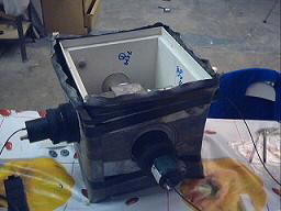
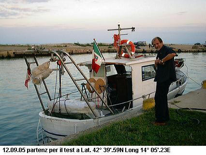
G. Giuliani acquista una vecchia barca da pesca destinata alla demolizione e da
tutti considerata non
più adatta alla navigazione.
Sotto la guida di un maestro d’ascia, dopo 6 mesi la vecchia barca viene
trasformata in un natante
laboratorio, per effettuare ricerche sul fondo marino sui medesimi precursori
sismici osservati sulla
terra ferma.
Come si presentava la barca prima del recupero, abbandonata in secca da 6
anni, in un piccolo
cantiere di Roseto Degli Abruzzi. 20 Aprile 2005. Stazza 4 Ton. L.f.t. 8m Semi
cab.
Motore BMV 3 Cil. 45CV.

Dopo un anno di preparativi e test effettuati al largo della costa Adriatica,
il 29 Aprile 2005, sono stati
registrati i primi dati acquisiti a 15 metri di profondità, a circa 5 miglia
dalla costa.
Di fianco la barca laboratorio dopo il restauro.
L’immagine mostra la barca prima della partenza, per gli ultimi test effettuati
al largo della costa
adriatica, tra Roseto e Giulianova.
Il prototipo rivelatore sottomarino utilizza la stessa tecnica dei rivelatori
di terra, l’unica differenza
riguarda l’ingegnerizzazione del detector, che prevede una tenuta stagna, per
operare su fondali marini
da 15m a 40m di profondità.
Il grafico sotto mostra le prime misure di Radon effettuate a 18 m di profondità
a circa 5 mgl dalla
costa tra Roseto (Te) e Giulianova (Te).
Dopo questi risultati si decise quindi di istallare una stazione di
rilevamento nella cittadina di Pineto
(Te) per correlare i dati ottenuti dalle stazioni di Coppito (Aq) e quella dei
Laboratori Nazionali Gran
Sasso in Assergi (Aq).
La stazione di Pineto, avrebbe effettuato correlazioni con i dati rilevati dalla
barca laboratorio al largo
della costa. Di fianco la barca laboratorio dopo il restauro.
L’immagine mostra la barca prima della partenza, per gli ultimi test effettuati
al largo della costa
adriatica, tra Roseto e Giulianova.
Questa ricerca sulle correlazioni tra il fondo del mare e la costa è a
tutt’oggi in corso, anche se, a
causa di mancanza di fondi, al momento subisce un forte rallentamento.
G. Giuliani.
Dal 16 gennaio scorso, chi abita nell'aquilano ha un pò la tremarella:.
Questo è il prospetto stralciato da gentili indicazioni dell'Istituto Nazionale
di Geofisica e Vulcanologia circa le scosse registrate nel mese di Febbraio
2009.
Data Ora Prof(Km) Mag Distretto Sismico
2009/02/17 18:13:06 9.6 Ml:2.4 Aquilano
2009/02/17 13:13:03 10.4 Ml:2.3 Aquilano
2009/02/17 06:08:34 9 Ml:2.6 Aquilano
2009/02/16 23:16:39 10.0 Mw:5.3 Ionian Sea
2009/02/16 18:43:08 124.8 Ml:2.7 Isole_Lipari
2009/02/16 12:41:53 10.4 Ml:1.8 Aquilano
2009/02/15 19:16:38 10.2 Ml:2.5 Aquilano
2009/02/15 07:41:40 11.5 Ml:2 Aquilano
2009/02/13 10:29:57 10 Ml:2.5 Aquilano
2009/02/13 06:39:13 8.6 Ml:3 Alta_Val_Tiberina
2009/02/12 12:12:58 68 Ml:2.7 Costa_siciliana_settetrionale
2009/02/11 17:34:53 33 Mw:7.5 Talaud Islands, Indonesia
2009/02/10 07:57:25 11.1 Ml:2.4 Prealpi_lombarde
2009/02/09 14:18:16 8.8 Ml:2.6 France
2009/02/07 08:02:35 6 Ml:3.4 Madonie
2009/02/05 22:29:48 5 Ml:2.4 Piana_del_Volturno
2009/02/05 17:43:55 10 Ml:2.8 Tirreno_centrale
2009/02/05 14:50:13 30.7 Ml:3.1 Mar_Ionio
2009/02/05 07:43:12 10 Ml:1.8 Irpinia
2009/02/05 03:55:22 22.8 Ml:3.2 Mar_Ionio
2009/02/04 16:57:32 10 Ml:2 Valle_del_Topino
2009/02/03 20:17:18 6.9 Ml:1.4 Garfagnana
2009/02/01 14:52:00 5.8 Ml:3.8 Mar_Ligure
2009/02/01 05:52:04 9.1 Ml:2.2 Aquilano
2009/02/01 00:57:09 35 Mb:4.8 Greece
+ altre sette trettecate nel mese di gennaio, degne di nota.
Sul sito www.ilcapoluogo.it, si dice però che l'Aquila dispone, "unica al
mondo", di un sofisticato sistema di "previsione dell'attività sismica",
brevettato nel 2003! da un geofisico aquilano.
"Il
"PM4", è una scatola pesante mezzo quintale, semplice come tutte le opere di
genialità, realizzata e brevettata da
Giampaolo Giuliani,
un tecnico aquilano in servizio presso i Laboratori Nazionali del Gran Sasso, e
prevede i terremoti in un ampio raggio d'azione e con un anticipo compreso tra
le 6 e le 24 ore, con una precisione molto alta. I precursori sismici vengono
incrociati con altre 4 stazioni così attrezzate che si trovano nella frazione di
Coppito, nei laboratori del Gran Sasso, nel vicino Comune di Fagnano e a Pineto
(Teramo). La triangolazione dei dati consente di individuare con una discreta
precisione epicentro e intensità di un evento sismico. Il sistema è stato
collaudato dal Dipartimento di Ingegneria delle strutture, delle acque e del
terreno (Disat) dell'Università dell'Aquila. I rivelatori - a differenza dei
sismografi, che non consentono di osservare un precursore sismico - percepiscono
l'energia di una faglia e si basano sull'analisi del decadimento del radon, gas
nobile con vita media 3,8 giorni: i 2 isotopi Piombo 214 e Bismuto 214 emettono
fotoni percepiti da uno scintillatore plastico e visualizzabili grazie a
fotomoltiplicatori, collocati in un cubo di piombo del peso di 6 quintali, con
pareti spesse 7 centimetri. Molte cose sono cambiate nel breve volgere di
qualche mese. I risultati raggiunti da Giuliani, dopo anni di studi, test e
lunghi esperimenti svolti a L'Aquila, erano regolarmente snobbati dalla scienza
ufficiale e dai geofisici. Secondo questi ultimi, prevedere i terremoti era
impossibile, ma la caparbia (e la precisione dei dati) del tecnico aquilano sta
gradualmente intaccando il muro di gomma eretto dagli scettici. L'ideatore del
"PM4" è entusiasta per i risultati registrati: "Abbiamo previsto tutti gli
eventi sismici con un'esattezza indiscutibile. La protezione civile riceve
regolarmente i nostri preallarmi e allarmi, emessi dai nostri rilevatori. Qui,
per adesso, vengono solamente analizzati dal tecnico
Roberto Ianni
il quale
ne controlla l'intensità. La scossa di ieri mattina (alle 7:08, magnitudo 2.6),
ad esempio, era stata preannunciata con un allarme della stazione di Coppito
alle 18 di ieri. Nell'ultimo mese le scosse avvertite nel territorio aquilano -
una o due al giorno - sono state puntualmente previste dalle stazioni gestite da
Giuliani il quale tranquillizza: "Il fatto che ci siano piccoli terremoti ogni
giorno non consente che si accumuli energia tale da scatenare un evento più
forte". Ma lo sciame sismico dura ininterrottamente da un mese, cosa sta
accadendo? "Il primo evento, ampiamente previsto dai nostri rilevatori, c'è
stato il 16 gennaio" spiega Giuliani."Da allora, escludendo un paio di giorni di
pausa sismica, ha scaricato praticamente tutti i giorni. Gli epicentri e
ipocentri più importanti sono sempre gli stessi e cioè Roio (località aquilana)
e la bassa valle dell'Aterno. Si tratta di uno sciame tellurico del tutto
normale - prosegue Giuliani - in quanto eventi simili si sono verificati anche
negli anni passati, ma quest'anno alcuni terremoti sono stati percepiti dalla
popolazione". Nel corso dei suoi studi sui terremoti, Giuliani e il suo staff
hanno monitorato 4.500 scosse sismiche registrate in tutta Italia, dalla Valle
d'Aosta a Pantelleria, giungendo a un'altra clamorosa scoperta: "Abbiamo notato
che la maggior parte dei terremoti si verificano durante i mesi invernali, o
meglio, quando il sistema terra-luna è nel perielio, quindi più vicino al sole.
In inverno, quando la terra subisce uno stress gravitazionale maggiore, si
registrano più eventi sismici (60-70%) che in estate. La percentuale si mantiene
ancora più alta quando c'è la luna nuova. Il magma che scorre sotto la crosta
terrestre risente delle attrazioni gravitazionali, come accade per gli oceani".
Giuliani ha fiducia sul fatto che la scoperta del secolo "made in L'Aquila"
possa dare lustro alla città: "Spero con tutto il cuore che i benefici che si
potranno trarre da questo brevetto restino a L'Aquila. Mi basta che il mondo
sappia di questa opportunità e che un domani, magari molto prossimo, si possano
divulgare le "previsioni sismiche" come accade per le previsioni metereologiche.
Tutto questo ci offre il lato per congedarci da Giuliani con la domanda che
tutti vorrebbero fargli: la popolazione civile sarà avvisata se il "PM4" dovesse
prevedere una scossa di forte intensità? "La gente - risponde - potrebbe essere
avvertita con 24 ore di anticipo e ci sarebbe tutto il tempo necessario per
premunirsi. Ma per arrivare a tale fine bisogna innanzitutto educare la
popolazione civile, e non solo". (di Luca Ceccarelli)
"
Angela Baglioni L'AQUILA
Il susseguirsi di scosse, anche se di bassa magnitudo, sta ormai diventando
una costante per il territorio aquilano. Nella giornata di ieri i sismografi
dell'Istituto nazionale di geofisica e vulcanologia di Roma hanno registrato
altri due terremoti. Il primo, di magnitudo 2, si è verificato alle 11,46. Il
secondo, pari a 2,4 gradi della scala Richter, è stato invece avvertito alle
13,11. Nella città dell'Aquila, ormai, serpeggia una vera psicosi e il ripetersi
frequente di movimenti tellurici non aiuta a tranquillizzare gli animi,
nonostante le rassicurazioni da parte della comunità scientifica. Tra l'altro,
ai terremoti veri si sono purtroppo aggiunte nei giorni scorsi notizie
allarmanti diffuse da un camioncino su presunte scosse distruttive, creando
notevole allarme tra la popolazione.
La Digos della Questura dell'Aquila, a questo proposito, ha avviato delle
indagini per tentare di risalire all'identità di coloro che, subito dopo i
terremoti più importanti, si sono "prodigati" nell'invitare la gente ad
abbandonare le rispettive abitazioni preannunciando scenari catastrofici.
Scenari, è bene ripeterlo, smentiti in maniera categorica dalla protezione
civile che a più riprese ha ribadito come alla luce delle attuali conoscenze
scientifiche non sia assolutamente possibile prevedere i terremoti. Fino a
questo momento sono state ascoltate due persone ma l'attività investigativa
prosegue. Eppure, ancora durante la giornata di ieri, circolavano voci
sull'allestimento di una tendopoli a Tornimparte, dove far "convergere" la
popolazione in caso di sisma. Anche questa notizia, ovviamente, non risponde al
vero ma testimonia il clima di quasi panico che ormai si è diffuso. Gli
investigatori non escludono il sospetto che qualcuno abbia interesse ad evacuare
le case per motivi non certo legati alla pubblica incolumità, ma più
prosaicamente per poter approfittare dell'assenza dei proprietari. Le forze
dell'ordine, comunque, non tralasciano alcuna pista, neanche quella della
goliardata di pessimo gusto. Nei giorni scorsi all'Aquila si è riunita la
commissione grandi rischi presieduta da Franco Barberi. Alla riunione, voluta
dal capo del dipartimento della protezione civile, Guido Bertolaso, hanno
partecipato tutte le componenti istituzionali coinvolte ai vari livelli. Tra gli
altri, erano presenti l'assessore regionale Daniela Stati e il sindaco
dell'Aquila, Massimo Cialente. Dopo l'incontro è stato
ribadito ancora il messaggio che non è possibile prevedere i terremoti.
Verosimilmente, hanno detto, è possibile ipotizzare lo scenario a partire dalle
caratteristiche geo-morfologiche del territorio. Di sicuro, non si potrà sapere
quando un evento sismico si verificherà. Lo sciame che interessa il territorio
aquilano e la conca di Sulmona va avanti ormai da più di tre mesi, con decine di
movimenti tellurici registrati dai sismografi. Nella sola giornata di lunedì
scorso, quando la sequenza ha raggiunto l'acme con la scossa di magnitudo 4, la
popolazione ha avvertito nell'arco di appena nove ore ben dieci terremoti. La
protezione civile mantiene alto il livello di attenzione anche se, come ribadito
dagli esperti, si tratta di una sequenza tutto sommato normale per un territorio
ad alto grado di sismicità, come quello aquilano. Il danno atteso, ha detto il
vice capo del dipartimento operativo nazionale di protezione civile, Bernardo De
Bernardinis a margine dell'incontro di martedì, non dovrebbe essere molto
diverso da quello che è stato determinato finora e che non ha tuttavia
interessato strutture portanti di edifici, salvo qualche rara eccezione dovuta
più che al terremoto a carenze gravi già note prima dell'avvio dello sciame
sismico. Il consigliere regionale del Pdci, Antonio Saia, nel frattempo, ha
presentato un'interrogazione per sapere quali provvedimenti intende assumere la
Giunta in relazione ai danni causati dagli eventi sismici e quali iniziative
saranno intraprese per ultimare la ricostruzione degli edifici danneggiati dal
terremoto di 25 anni fa.
A L'Aquila la prima sala di previsione sismica
al mondo

E' esecutiva dall'agosto del 2008 e
funziona perfettamente la prima stazione di previsione dei terremoti esistente
al mondo.
Lo sciame sismico che dal 16 gennaio scorso
sta interessando la città dell'Aquila è la circostanza ideale per testarne
l'attendibilità. Lo abbiamo fatto andando a trovare chi ha realizzato e
brevettato il "PM4", una magica scatola di piombo
che permette di prevedere un evento sismico dalle 6 alle 24 ore prima
dell'evento.
La "sala sismica" per la previsione di terremoti è stata
attrezzata all'interno della scuola elementare "De Amicis", a San Bernardino,
grazie alla concessione di alcuni locali da parte del Comune dell'Aquila
che, assieme al dirigente provinciale Francesco Bonanni e al
direttore dei Laboratori
del Gran Sasso d'Italia, Eugenio Coccia, hanno prestato fede e
scommesso sull'invenzione di Giuliani.
Il "PM4", è una scatola pesante mezzo quintale, semplice come tutte le opere di
genialità, realizzata e brevettata da Giampaolo Giuliani,
un tecnico aquilano in servizio presso i Laboratori Nazionali del Gran Sasso, e
prevede i terremoti in un ampio raggio d'azione e con un anticipo
compreso tra le 6 e le 24 ore, con una precisione molto alta.
I precursori sismici vengono incrociati con altre 4 stazioni così attrezzate che
si trovano nella frazione di Coppito, nei laboratori del Gran Sasso,
nel vicino Comune di Fagnano e a Pineto (Teramo). La triangolazione dei dati
consente di individuare con una discreta precisione epicentro e intensità di un
evento sismico.
Il sistema è stato collaudato dal Dipartimento di Ingegneria delle strutture,
delle acque e del terreno (Disat) dell'Università dell'Aquila.
I rivelatori - a differenza dei sismografi, che non consentono di osservare un
precursore sismico - percepiscono l'energia di una faglia
e si basano sull'analisi del decadimento del radon, gas nobile con vita media
3,8 giorni: i 2 isotopi Piombo 214 e Bismuto 214 emettono
fotoni percepiti da uno scintillatore plastico e visualizzabili grazie a
fotomoltiplicatori, collocati in un cubo di piombo del peso di 6 quintali,
con pareti spesse 7 centimetri. Il brevettatore del sistema (brevettato nel
2003) è l'aquilano Gioacchino Giampaolo Giuliani,
tecnico di ricerca dell'Inaf (Istituto Nazionale di Astrofisica),
associato Infn (Istituto Nazionale di Fisica Nucleare),
che dal 2002 ha speso tutte le sue energie sulla realizzazione di un sistema di
previsione dei terremoti dopo aver riscontrato
che l'andamento del flusso di radon, un gas naturale, è strettamente legato ad
un evento sismico.
Molte cose sono cambiate nel breve volgere di qualche mese. I risultati
raggiunti da Giuliani, dopo anni di studi, test e lunghi esperimenti svolti a
L'Aquila,
erano regolarmente snobbati dalla scienza ufficiale e dai geofisici. Secondo
questi ultimi, prevedere i terremoti era impossibile,
ma la caparbia (e la precisione dei dati) del tecnico aquilano sta gradualmente
intaccando il muro di gomma eretto dagli scettici.
L'ideatore del "PM4" è entusiasta per i risultati registrati: "Abbiamo previsto
tutti gli eventi sismici con un'esattezza indiscutibile.
La protezione civile riceve regolarmente i nostri preallarmi e allarmi, emessi
dai nostri rilevatori. Qui, per adesso, vengono solamente
analizzati dal tecnico Roberto Ianni il quale ne controlla
l'intensità. La scossa di ieri mattina (alle 7:08, magnitudo 2.6), ad esempio,
era stata preannunciata con un allarme della stazione di Coppito alle 18 di
ieri. Nell'ultimo mese le scosse avvertite nel territorio aquilano
- una o due al giorno - sono state puntualmente previste dalle stazioni gestite
da Giuliani il quale tranquillizza:
"Il fatto che ci siano piccoli terremoti ogni giorno non consente che si
accumuli energia tale da scatenare un evento più forte".
Ma lo sciame sismico dura ininterrottamente da un mese, cosa sta accadendo?
"Il primo evento, ampiamente previsto dai nostri rilevatori, c'è stato il 16
gennaio? spiega Giuliani.
"Da allora, escludendo un paio di giorni di pausa sismica, ha scaricato
praticamente tutti i giorni.
Gli epicentri e ipocentri più importanti sono sempre gli stessi e cioè Roio e la
bassa valle dell'Aterno.
Si tratta di uno sciame tellurico del tutto normale - prosegue Giuliani - in
quanto eventi simili
si sono verificati anche negli anni passati, ma quest'anno alcuni terremoti sono
stati percepiti dalla popolazione".
Nel corso dei suoi studi sui terremoti, Giuliani e il suo staff hanno monitorato
4.500 scosse sismiche registrate in tutta Italia,
dalla Valle d'Aosta a Pantelleria, giungendo a un'altra clamorosa scoperta:
"Abbiamo notato che la maggior parte dei terremoti
si verificano durante i mesi invernali, o meglio, quando il sistema terra-luna è
nel perielio, quindi più vicino al sole.
In inverno, quando la terra subisce uno stress gravitazionale maggiore, si
registrano più eventi sismici (60-70%) che in estate.
La percentuale si mantiene ancora più alta quando c'è la luna nuova. Il magma
che scorre sotto la crosta terrestre risente
delle attrazioni gravitazionali, come accade per gli oceani".
Giuliani ha fiducia sul fatto che la scoperta del secolo "made in L'Aquila"
possa dare lustro alla città:
"Spero con tutto il cuore che i benefici che si potranno trarre da questo
brevetto restino a L'Aquila.
Mi basta che il mondo sappia di questa opportunità e che un domani, magari molto
prossimo,
si possano divulgare le "previsioni sismiche" come accade per le previsioni
metereologi che.
Tutto questo ci offre il lato per congedarci da Giuliani con la domanda che
tutti vorrebbero fargli: la popolazione civile sarà avvisata se il "PM4"
dovesse prevedere una scossa di forte intensità? "La gente - risponde - potrebbe
essere avvertita con 24 ore di anticipo e ci sarebbe tutto il tempo
necessario per premunirsi. Ma per arrivare a tale fine bisogna innanzitutto
educare la popolazione civile, e non solo".
Altro articolo:
Giampaolo Giuliani utilizza il Radon, un gas
nobile emesso dalla crosta terrestre. Lo stesso nome e’ stato dato al suo
apparecchio che dovrebbe prevedere i sismi.
Ma la protezione civile
smentisce che lui ci riesca. Lui e’ convinto di aver creato l’oggetto giusto
per prevedere tante catastrofi. Per questo i suoi cubi ora sono sparsi
per l’Abruzzo: nel 2004 reagirono anche con largo anticipo al sisma che causo lo
Tsunami in Indonesia.
Domenica Giampaolo Giuliani ha previsto una violenta scossa nel
pomeriggio, dopo quella della mattina, a Sulmona. Subito il fisico ha chiamato
la polizia e il sindaco,
che si trovava a Roma al congresso del Popolo della Libertà. Peccato che il
terremoto non si sia mai verificato. E con la sua
falsa previsione ha causato un caos allucinante.
Tanto che ora e’ stato denunciato per aver creato falso allarmismo.
Il sindaco commenta cosi’: “Non è possibile che si vada in giro a creare
allarmismi, domenica ho passato la giornata più brutta della mia vita perché
dopo aver parlato con quel signore, che mi aveva annunciato un sisma devastante,
molto più forte di quello che c’era stato in mattinata, mi sono trovato in una
situazione difficilissima. Perché non sapevo che cosa fare: far scattare il
piano di evacuazione o far finta di niente, con il rischio di portarmi sulla
coscienza una possibile tragedia?“.
Ma Giampaolo Giuliani va avanti con il suo lavoro: lui e’ convinto che i suoi
cubi dicano il vero!
Previsione analitica e non pronostico calcistico o
profezia come e' stato scritto da alcuni.
Scosse sismiche Aquila: Gennaio, Febbraio, Marzo.
Viste le numerose richieste degli utenti riportiamo la tabella delle scosse
sismiche rilevate a L’Aquila e provincia, negli ultimi 4 mesi.
Sono dati puramente informativi dei quali non possiamo
garantire l’assoluta correttezza.
la prima colonna riporta la data e l’ora in tempo locale.
la seconda colonna il magnitudo
la terza colonna la profondità dell’evento in chilometri
la quarta colonna la provincia interessata
| 26/03/2009 03:10:38 |
2 |
11 |
L Aquila |
| 24/03/2009 09:27:54 |
1.8 |
10 |
L Aquila |
| 22/03/2009 08:02:55 |
2.3 |
10 |
L Aquila |
| 18/03/2009 10:23:09 |
2.2 |
9 |
L Aquila |
| 13/03/2009 16:29:55 |
2.4 |
10 |
L Aquila |
| 13/03/2009 14:49:14 |
1.8 |
9 |
L Aquila |
| 13/03/2009 14:09:52 |
1.3 |
5 |
L Aquila |
| 11/03/2009 22:55:49 |
2.9 |
9 |
L Aquila |
| 10/03/2009 12:25:27 |
2.2 |
10 |
L Aquila |
| 22/02/2009 08:03:40 |
1.3 |
12 |
L Aquila |
| 21/02/2009 18:04:10 |
2.2 |
10 |
L Aquila |
| 17/02/2009 19:13:06 |
2.4 |
10 |
L Aquila |
| 17/02/2009 14:13:03 |
2.3 |
10 |
L Aquila |
| 17/02/2009 07:08:34 |
2.6 |
9 |
L Aquila |
| 16/02/2009 13:41:53 |
1.8 |
10 |
L Aquila |
| 15/02/2009 20:16:38 |
2.5 |
10 |
L Aquila |
| 15/02/2009 08:41:40 |
2 |
12 |
L Aquila |
| 13/02/2009 11:29:57 |
2.5 |
10 |
L Aquila |
| 01/02/2009 06:52:04 |
2.2 |
9 |
L Aquila |
| 31/01/2009 00:00:01 |
2.3 |
10 |
L Aquila |
| 30/01/2009 22:54:19 |
2.5 |
10 |
L Aquila |
| 30/01/2009 01:39:03 |
2.5 |
9 |
L Aquila |
| 24/01/2009 10:06:07 |
2.4 |
10 |
L Aquila |
| 23/01/2009 19:51:56 |
2 |
8 |
L Aquila |
| 18/01/2009 09:13:43 |
2.1 |
9 |
L Aquila |
| 16/01/2009 23:47:23 |
2.4 |
11 |
L Aquila |
| 14/12/2008 09:00:00 |
1.8 |
10 |
L Aquila |
fonte dei dati: European-Mediterranean Seismological Centre
PROGETTO DI MASSIMA DI UN SISTEMA DI MONITORAGGIO PER LA PREVISIONE
SISMICA ED ADATTABILE SU QUALSIASI TERRITORIO AD ALTO RISCHIO SISMICO.
Ogniqualvolta si verifica una calamità naturale, ci si ricorda della fragilità
del pianeta su cui
viviamo.
Ci si rende conto della drammaticità dell’evento, nel momento in cui si contano
le vittime, si
raccolgono i feriti e si calcolano i danni ingenti.
Trascorsa la crisi, ci si dimentica dei disagi delle popolazioni colpite, dei
danni ingenti, delle vite
umane perdute, del gran numero di invalidi che restano.
Alcuni dati degli ultimi forti terremoti:
16 Agosto 1999 11:11 terremoto M = 7.8 a IZMUT (Turchia), morti ≈ 10.000, Feriti
45.000.
26 Gennaio 2001 03:16 terremoto M = 7.9 Gujarat (India), morti > di 20.000.
21 Maggio 2003 18:44 terremoto M = 6.7 ALGERIA morti ≈ 2000, feriti 6782.
26 Dicembre 2003 01:56 terremoto M = 6.3 Bam (Iran), morti ≈ 40.000 (Bam
distrutta)
24 Dicembre 2004 terremoto M = 9.2 Indonesia e area asiatica morti > di 180.000.
Costo dei danni incalcolabili.
La Sezione Ricerca della S.C.S. (Società di collaborazioni Scientifiche) ha
realizzato nel 2002 un
sistema che permette di registrare allarmi sismici con un margine di anticipo
sull’evento da 6 ore
a 24 ore. Il sistema è stato brevettato in Italia con n. 0001333804 a nome del
Sig. Gioacchino
Giuliani.
L’installazione di un sistema di monitoraggio per la previsione di eventi
sismici, fornito dalla
S.C.S., trova applicazione presso qualsiasi territorio terrestre ad alto rischio
Sismico.
Il sistema si avvale dell’applicazione di una rete di rivelatori di gas Radon,
distribuita sul territorio
o regione prescelta per il monitoraggio.
La rete di rivelatori del tipo PM4 e PM2, forniscono allarmi sismici con un
margine di anticipo
sull’evento da 6 a 24 ore prima di un terremoto.
Il metodo utilizzato dai rivelatori del tipo PM4 e PM2, permette di rilevare il
flusso medio del gas
Radon ed attraverso un’analisi del continuo dello stesso gas di rilevare quei
segnali considerati
precursori sismici, che vengono prodotti da 6 a 24 ore prima di un evento
sismico.
L’intera rete di monitoraggio sarà costituita da una serie di punti nodali
distribuiti lungo il territorio
destinato al controllo della sismogeneticità della zona prescelta.
Ogni nodo dell’intera rete di monitoraggio, è costituito da almeno tre
rivelatori del tipo PM4 e
PM2, posti ad una distanza fra loro pari ad un minimo di 25 Km ad un massimo di
80 Km.
La distanza tra i rilevatori nodali è determinata dalla natura del territorio e
dalla sismogeneticità dei
luoghi da sottoporre a monitoraggio.
Ogni rivelatore di Radon, (PM4 o PM2) costituirà quindi una Stazione di
rilevamento ed
acquisizione dati.
Le varie stazioni dei diversi punti nodali, saranno tra loro interallacciate e
collegate ad una Sala
Sismica Centrale.
I dati forniti dalle singole stazioni e gli allarmi sismici provenienti dai
diversi punti nodali,
convergeranno sui monitors della Sala Sismica Centrale.
L’allarme sismico prodotto dai punti nodali, sarà costituito da un messaggio
e-mail contenente
l’informazione sulla stazione o stazioni che hanno inviato l’allarme, le
coordinate della località
dove è previsto l’evento ed il valore del grado sismico richter previsto.
Un messaggio telefonico può essere inviato nello stesso tempo ad un utente
addetto al controllo
degli allarmi.
L’eventuale allarme di grado richter considerato pericoloso per la popolazione
della regione
interessata, sarà gestito da personale dell’ente preposto alla diffusione delle
informazioni sugli
allarmi sismici.
Naturalmente il sistema di gestione degli allarmi sismici, prevede un periodo di
specializzazione da
parte del personale preposto al controllo della sala sismica, al controllo degli
allarmi delle singole
stazioni ed all’analisi dei dati provenienti dai vari punti nodali.
Ogni stazione di rilevazione, che dovrà ospitare un rivelatore di tipo PM4 o
PM2, necessita di una
piccola stanza, interrata o semi interrata, senza ventilazione o possibilità di
scambi di aria con
ambienti diversi da quello destinato all’alloggiamento del rivelatore.
Il locale in questione necessita di un punto presa per la corrente elettrica
220/250 Volts ed un punto
presa di collegamento alla rete internet.
Ogni rivelatore ha un ingombro medio di 70 cm x 70 cm x 70 cm.
Il peso del rivelatore può variare da 400 Kg a 500 Kg.
L’ingombro dell’elettronica di acquisizione ed analisi per una stazione sarà
pari a 70 cm x 70 cm x
100 cm h. Peso dell’elettronica da 40 Kg a 60 Kg.
La potenza elettrica impegnata per l’alimentazione di una stazione, è pari a
1000 W.
La S.C.S. provvederà all’istallazione dei rivelatori, al controllo degli stessi
ed all’allestimento della
Sala Sismica di controllo.
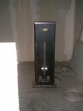
A titolo di esempio vengono di seguito riportate immagini del rivelatore,
dell’elettronica e delle
mappe cartografiche raffiguranti il tipo di rete di monitoraggio.
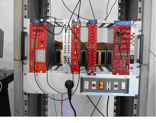
Esempio di ingombro del tipo di elettronica utilizzato per una stazione di
monitoraggio, per il
rilevamento della variazione di concentrazione di Radon.
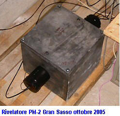
Rivelatore di tipo PM2, utilizzato in una stazione di monitoraggio per la
rivelazione del flusso
medio della concentrazione di Radon in ambiente.
Esempio di piccola rete di monitoraggio in Abruzzo. Costituita da n. 3
rivelatori di Tipo PM4 e
PM2. Le Stazioni operative rappresentate sono quelle di L’Aquila, Gran Sasso (Assergi)
e
Pineto (TE)
Rivelatore di tipo Pm4 attualmente operativo presso la stazione di
rivelamento Coppito (L’Aquila)
Esempio di una grande rete di monitoraggio, per la previsione sismica.
Studio effettuato dalla S.C.S. per un territorio ad altissimo rischio sismico,
utilizzando mappe
sismogenetiche, relative ad una area attraversata da una grande faglia.
La relazione descritta è stata curata dai Sig.ri Gioacchino Giuliani e
Roberto Giuliani, per conto
Della S.C.S.
Società di Collaborazioni Scientifiche
Via del Corso, 29/31
67110 L’Aquila – Italy
Tel. 00390862362813
Cell. 00393389798972.
Altro articolo
Due tecnici Aquilani ed un amico Russo, Giampaolo Giuliani, Roberto Giuliani
e Victor Alekseenko potrebbero cambiare il mondo e la nostra città
L'Aquila, 9 nov. - "...e ora passiamo alle previsioni sismiche; prevista una
leggera scossa sismica per domani pomeriggio nella zona di Los Angeles." Non
si tratta di una scena da film futuristico hollywoodiano, ma di una realtà
molto vicina, anzi, a L'Aquila già operativa. Si chiama "PM4", è una scatola
pesante mezzo quintale, semplice come tutte le opere di genialità,
realizzata e brevettata da Giampaolo Giuliani, un tecnico aquilano in
servizio presso i Laboratori Nazionali del Gran Sasso, e prevede i terremoti
in un ampio raggio d'azione e con un anticipo compreso tra le 6 e le 24 ore,
con una precisione molto alta. La eclatante notizia risale al 2003 e fu
anticipata dal nostro direttore Gianfranco Colacito sulle pagine
dell'Opinione, poi scese il silenzio... (segue)
"I tempi erano forse prematuri" - ci spiega Giuliani - "da quando Colacito
pubblicò quel bellissimo articolo, ho dovuto subirne tante". Ma andiamo per
ordine. Siamo andati a trovare Giampaolo Giuliani dopo aver appreso che
l'Istituto di Fisica Nucleare del Gran Sasso, pur non prendendo parte
direttamente alla sperimentazione, ha deciso di installare uno dei
macchinari "MP4" per testarne l'efficacia. Entriamo nel laboratorio privato
di Giuliani, Presso la Ditta S.C.S. di Coppito, "CHIOCCIOLANDIA", ed è come
ci aspettavamo che fosse: una specie di officina artigianale con macchinari
scintillanti di lucette e computer, non certo gli avveniristici laboratori
con gli effetti speciali o scansioni laser dell' iride per accedere nelle
segrete sale della scienza ufficiale. Solo lavoro, passione e genialità. La
prima domanda è logica: "Ha scoperto una macchina del genere e il mondo non
sa nulla? Funziona davvero o è una sperimentazione?" - "Altrochè se
funziona, e già da qualche anno! Non è semplice spiegare tutto. Non sono uno
scienziato, sono soltanto un tecnico che ha scoperto "l'uovo di Colombo". La
scienza ufficiale è convinta che non si possano prevedere i terremoti, e
potete immaginare a quanti incontri-scontri con l'elite scientifica ho
dovuto far fronte. Ma i dati e i rilevamenti che ho sono inconfutabili". -
La solita vecchia storia, dunque, quando per la Scienza non è piacevole
comprendere che si è insegnato per anni qualcosa di inesatto come ad esempio
la teoria tolemaica, e dover cominciare a ridisegnare teorie e studi. L'MP4
è stato ideato e costruito da Giuliani con l'aiuto del figlio Roberto, del
fisico russo Victor Alekseenkor e di pochi altri collaboratori ed è
brevettato a livello nazionale ed internazionale. La tecnica utilizzata si
basa sulla rilevazione del radon 222, un gas radioattivo, da cui il
Rivelatore evidenzia alcuni figli diretti della catena di decadimento
radioattivo (così li chiama Giuliani) e da cui un software specifico
seleziona i così detti Precursori Sismici, quando i precursori vengono
rivelati, un particolare algoritmo sempre via software provvede a lanciare
un Preallarme o un Allarme dalle 6 alle 24 ore prima dell'evento.
Con almeno tre rivelatori distanti fra loro un certo numero di Km. Sarà
possibile dare anche la prossimità dell'epicentro ed il grado sismico.
Abbiamo superato con successo tutti i test e in quattro anni abbiamo
previsto praticamente tutti i terremoti rilevati dall'MP4, con una
efficienza fuori dalle attese. La scoperta di Giuliani è consistente e di
portata mondiale, tanto è vero che Eduard Nixon, fratello dell'ex presidente
degli Stati Uniti, attualmente capo della Protezione civile di San
Francisco, ha chiesto finanziamenti al governatore per l'acquisto di 5
detector. Attualmente vi sono in funzionamento 2 rilevatori, uno a L'Aquila
ed uno a Pineto. Il team di Giuliani è stato inoltre il primo al mondo ad
effettuare rilevamenti di radon sul fondo del mare al largo delle coste
abruzzesi ottenendo risultati inattesi. E ora la nota dolente.
L'Aquila rischia di perdere ancora una volta una possibilità enorme
dal momento che nessuno è stato in grado di afferrarne le
enormi possibilità. In un territorio che perde ogni giorno posti di lavoro
si presenta una specie di miracolo che potrebbe portarci all'attenzione
mondiale. Giuliani da aquilano verace ed un po' campanilista vorrebbe che
sia L'Aquila e l'Abruzzo a beneficiare dei frutti che potrebbero scaturire
dalla scoperta, una volta che avrà ottenuto l'ufficialità anche dal mondo
scientifico. Il rischio di vedere trasportata altrove un'azienda che produca
migliaia di questi macchinari è alto.
In Italia sono già pronte molte città che farebbero salti mortali per
produrre il brevetto, oltre che, naturalmente, le grandi potenze americane,
russe e giapponesi. -
ROMA - Giampaolo Giuliani, il tecnico denunciato
per procurato allarme dopo aver previsto che un terremoto di grande entità
avrebbe potuto colpire la zona di L'Aquila,
era stato intervistato il 24 marzo anche dal blog DonneDemocratiche.it.
Nell'intervista, dopo aver raccontato com'è nato il suo apparecchio, aveva
corretto la sua prima previsione,
dicendo: "Mi sento di poter tranquillizzare i miei concittadini". In un'altra
intervista, rilasciata ad una tv locale, ora visibile su You Tube e sul sito di
Repubblica.it, era stato più determinato
e aveva detto che una rete di "precursori" potrebbe garantire una capacità
predittiva di grande rilevanza umana e sociale.
Sulle sue dichiarazioni, che in queste ore fanno il giro dei mezzi di
informazione, si sta scatenando una polemica, se è vero che l'Istituto di
Geofisica e Vulcanologia ribadisce oggi in un comunicato ufficiale: "Si
sottolinea la circostanza secondo la quale, allo stato attuale delle conoscenze,
non è possibile realizzare una previsione deterministica dei terremoti
(previsione della localizzazione, dell'istante e della forza dell'evento). Ciò è
vero anche in presenza di fenomeni quali sequenze o sciami sismici che nella
maggior parte dei casi si verificano senza portare al verificarsi di un forte
evento. Una scossa quale quella che si è manifestata oggi viene normalmente
seguita da numerose repliche, alcune delle quali probabilmente assai sensibili."
Nell'intervista a DonneDemocratiche, Giuliani specifica che il suo "precursore
sismico" arriva ad anticipare il verificarsi di un terremoto fino a 6-24 ore
prima.
La tecnica è basata sullo studio del "comportamento" dell'elemento chimico
chiamato Radon. Ecco il racconto di Giuliani: "Nel 2001 stavamo osservando il
misuratore di particelle cosmiche presso l'Istituto quando, in corrispondenza
del terremoto in Turchia, rilevammo una quantità straordinaria, rispetto al
solito, di radon. Così ho impiegato quasi 2 anni per realizzare da solo uno
strumento in grado di rilevare il radon, iniziai ad osservarlo ed a studiarlo, e
con l'aiuto di un sismografo mi resi conto che la concentrazione di radon
aumentava in corrispondenza di un evento sismico. Nel 2002, ad esempio, in
corrispondenza del terremoto di S. Giuliano, registrammo valori 100 volte
maggiori alla norma, ma disponendo di 1 solo precursore sismico eravamo in grado
di emanare un allarme per un evento sismico che distava più di 50 km da
L'Aquila, senza poter fornire altre informazioni circa la collocazione o la
direzione dell'evento stesso. Oggi con 5 precursori saremmo in grado di essere
molto più precisi, triangolando i dati ed i segnali di concentrazione del radon"
Dopo aver fornito elementi utili sulle caratteristiche del Radon, Giuliani dice
che il suo apparecchio non si trova nel campo della teoria, me ne esistono già
cinque esemplari:" "I 5 Precursori sismici si trovano a Coppito, nel Laboratorio
del Gran Sasso (ospite dell'INFN), presso la scuola De Amicis, a Fagnano e a
Pineto; sono tutti a più di 3 metri sotto terra e in corrispondenza di un evento
sismico rilevano nello stesso momento, lo stesso segnale creando un grafico
perfettamente sovrapponibile."
Poi Giuliani entra nel merito degli allarmi che si sono verificati in Abruzzo e
della sua previsione: "I dati ottenuti in questi 9 anni di studi, ci hanno
consentito di rilevare un rischio sismico maggiore nel periodo invernale che va
da novembre ad aprile. Senza voler banalizzare, ma per semplificare i concetti,
posso aggiungere anche che l'attività sismica è strettamente correlata alle fasi
lunari. In particolare quest'anno, il sistema Terra-Luna, si è venuto a trovare
al Perielio (punto più vicino al Sole, in inverno) con la Luna nello stesso
periodo alla minima distanza dalla Terra, e con il Pianeta Venere allineato, in
fase di Venere piena anch'essa vicina. L'attrazione gravitazionale delle masse
sulla Terra hanno intensificato l'effetto marea sul nostro pianeta, rendendo gli
eventi sismici più rilevanti, rispetto agli altri sciami, cui siamo stati
interessati negli anni precedenti. Mi sento di poter tranquillizzare i miei
concittadini, in quanto lo sciame sismico andrà scemando con la fine di marzo."
Ma evidentemente il metodo non è ancora accettato uniformemente. Giuliani
descrive così l'atteggiamento della comunità scientifica: "Mi osserva con
interesse ... una parte mi da fiducia, come dimostra anche il Direttore dell'INFN
che mi ha messo a disposizione un locale per ospitare uno dei 5 Precursori
sismici; una parte è un po' più cauta e scettica."GIAMPAOLO gIULIANI
RIBADISCE: LA DENUNCIA: «SI POTEVA CAPIRE» - Oggi, dopo la tragedia,
Giuliani parla con amarezza: «C'è il rischio che domani mi mettano in galera -
dice - ma confermo: non è vero, è falso, che i terremoti non si possono
preveder. Sono 10 anni che noi riusciamo a prevedere eventi di questo tipo in
una distanza di 100-150 chilometri da noi. Da tre giorni - continua- vedevamo un
forte aumento di radon, al di fuori della soglia di sicurezza. E forti aumenti
di radon segnalano forti terremoti. Questa notte il mio sismografo denunciava
una forte scossa di terremoto e ce l'avevamo online. Tutti potevano osservarlo e
tanti l'hanno osservato. Poteva essere visto ce ci fosse stato qualcuno a
lavorare o si fosse preoccupato. Abbiamo vissuto la notte più terribile della
nostra vita, sono sfollato anche io... Questi scienziati canonici, loro lo
sapevano che i terremoti possono essere previsti».
Altro Articolo:
 Ecco il tracciato del Sisma che ha
colpito l'Aquila, di magnitudo 5.8
Ecco il tracciato del Sisma che ha
colpito l'Aquila, di magnitudo 5.8
La Rete
Sismica Nazionale dell’INGV ha registrato un terremoto di Magnitudo 5.8
(Magnitudo Richter) (6.2 Mw=magnitudo momento) nella zona dell'Aquilano, il 6
Aprile 2009 alle 3:32 (ora italiana). Le coordinate epicentrali risultano le
seguenti: Lat. 42.33N e Long. 13.33 E. La
profondità dell'ipocentro è pari a 8.8 km. Il terremoto è caratterizzato da un
meccanismo di tipo estensionale, con piani di faglia orientati NW-SE e direzione
di estensione NE-SW (anti-appenninica)".
Nell'articolo
Portali-addendum, si legge: "Il Gran Sasso, cui accennai in
Portali (prima parte), si trova più o meno sulla stessa longitudine (13
gradi e 34 primi) di Lipsia (12 gradi e 23 primi). In
laboratori ricavati nel cuore della montagna, non si studierebbero solo
neutrini, ma si compirebbero esperimenti segreti. Alcuni scalatori hanno
affermato di aver colà notato anomalie".
La longitudine del sisma coincide quasi perfettamente con quella in cui è
ubicato il laboratorio sotterraneo. Ora, con i dati a nostra disposizione, non è
possibile stabilire se la scossa sia stata naturale o artificiale. Stando ad
alcuni ricercatori, un terremoto generato da sistemi d'arma come H.A.A.R.P. è
contraddistinto da una frequenza più alta.
Secondo la scienziata statunitense Rosalie Bertell, armi elettromagnetiche “sono
in grado di causare terremoti in siti scelti come bersaglio, sprigionando
energie equivalenti alle più forti esplosioni nucleari”.
E' possibile che il fenomeno tellurico sia stato prodotto da movimenti delle
faglie: infatti "l’attività di questi giorni si colloca tra la terminazione
meridionale della faglia che si è attivata nel terremoto del 1703 (Int. MCS del
X grado MCS, pari a Magnitudo circa 6.7) ed i limiti settentrionali della faglia
associata nei cataloghi al terremoto del 1349 e di quella denominata 'Ovindoli-Piani
di Pezza'”.
Comunque sia, è sintomatico che la "scienza" ufficiale si ostini a dichiarare
che i sismi non possono essere in nessun modo preveduti. Giampaolo Giuliani ed
altri dissentono. (Si ascolti l'intervista che riporta you tube sull'argomento).
E' inammissibile che tristi personaggi come Guido Bertolaso osino denunciare per
procurato allarme (sic) chi avverte circa possibili pericoli. Cassandra andrebbe
ascoltata, mentre gli incompetenti (ammesso e non concesso che si tratti solo di
incompetenza) meritano inesorabile riprovazione.
Ci chiediamo a che cosa servano i tanto decantati "progressi scientifici", se
ancora non si riesce a predire con una buona approssimazione eventi tanto
disastrosi. Come spesso avviene, quasi tutte le innovazioni riguardano gli
apparati militari. Forse evitare che un terremoto provochi danni e vittime non è
nell'interesse dei governi: alcuni
geologi d'altronde, invece di adoperarsi per monitorare la
situazione sismica, invece di compiere studi utili per la collettività,
preferiscono indagare le scie di "condensazione".
Secondo Angelo Ciccarella,
la città di Lipsia, nell'ex Germania est si può considerare un portale.
Nell'articolo intitolato La faccia occulta del Comunismo, lo studioso
riferisce di audaci e pericolosi esperimenti compiuti dalla Stasi,
la famigerata polizia segreta della Repubblica "democratica" tedesca, nel centro
militare di Lipsia.
L'autore scrive: "Ad un certo punto degli esperimenti collettivi, qualcosa
avvenne, qualcosa di terribile si rivelò.
Un arco di radiazioni elettromagnetiche in espansione saliva attraverso gli
strati delle vecchie e mai perdute trasmissioni radio di tutto il mondo.
Mentre l'arco procedeva in avanti nello spazio, viaggiava indietro nel tempo e
tutti i sensitivi, i tecnici, gli agenti Stasi presenti nel laboratorio,
ascoltarono voci di persone morte da tempo, fino a tornare verso la prima
trasmissione di Marconi e... verso il silenzio.
Poi, di botto, una cascata inarrestabile di fenomeni:
onde scalari, anomali flussi
energetici, ampio spettro di frequenze E.M. e nota di fondo dominante,
fragorosa. Uno squarcio nel vuoto ed ecco comparire un grande arazzo sopra le
teste dei presenti. Vi era raffigurato un animale, una salamandra in mezzo alle
fiamme.
Si era creato un punto cieco, un varco dimensionale. Inavvertitamente, pigiando
un tasto, oltre lo specchio si era acceso un led. Le facoltà extrasensoriali
di uomini e donne unite ad un glifo psicoacustico ed ad un codice alieno (?)
avevano trapassato le Porte del Tempo. La Quarta dimensione non è impenetrabile.
Quando si lacera la sua struttura connettiva, ne sopravviene un universo
tangente, instabile, limitato nella trasmissione. Esisterebbero così infiniti
universi, nei quali si svilupperebbero, in maniera indipendente, tutte le
alternative possibili, a partire da una situazione che ha la possibilità di
evolvere in diversi modi... Ciascuna alternativa diventerebbe così realizzata e
praticabile in un mondo a sé, senza essere cancellata dalle altre nelle vicende
di un unico mondo... Lipsia era un cancello stellare che attendeva da tempo di
essere aperto, un dispositivo in grado di viaggiare nel tempo e nelle
dimensioni. I massimi esperti di fisica e di elettronica provarono inutilmente
ad usare il portale come arma. Il portale da solo non serve a nulla; per
funzionare ha bisogno di un suo omologo di uscita nel segmento spazio-temporale
di arrivo. Indovinate dove si trova l'altra porta e soprattutto chi la detiene?"
Ciccarella intravede dietro le quinte della storia una cospirazione di
proporzioni gigantesche: il nome in codice dell’Entità che agisce nell’ombra è
Salamandra.
La salamandra, animale che, nella tradizione, era in grado di vivere nel fuoco,
ricorda le figure create dal plasma.
Nel suo testo criptico, non privo di autocompiacimento e di qualche tono da
ierofante, Ciccarella ha comunque il merito di rispolverare gli inquietanti
scenari di un conflitto segreto, il conflitto delle psicospie. Durante gli anni
della Guerra fredda, agenti psichici statunitensi (famoso è lo scienziato ed
artista Ingo Swann) e dell'est europeo si confrontarono in esperimenti di
visione a distanza ed in altri ambiti relativi all'uso a fini spionistici dei
poteri mentali. L'ipotesi dell'autore pare la seguente: forze extrasensoriali
furono all'origine di un'apertura nella sfera spazio-temporale. E' probabile che
ai risultati concorsero diaboliche tecnologie. La convergenza tra dimensione
medianica e tecnologica sembra essere all'origine delle scoperte che resero
celebre Marconi; un ascolto di esseri dell'altrove illuminò la mente di
Tesla. Gli scientisti reputano tale approccio ridicolo, poiché essi
distinguono tra la scienza e la superstizione. Sappiamo, però, quanto le
ricerche di eminenti studiosi anche razionalisti siano venate di magia, di
occultismo.
La riflessione sui portali, su questi aditi verso regioni invisibili ci conduce
al confine della percezione ordinaria, là dove i concetti razionali si appannano
per compenetrarsi con idee controintuitive, con i paradossi delle verità
eccentriche ed inaccettabili, appena rasentate da intelletti sublimi. Quando ci
accostiamo a certe verità mai attinte prime, esse si sbriciolano e si
depauperano, a contatto con il linguaggio e la logica.
Dove potrebbe essere l'altra porta verso l'Ade? Forse nelle viscere del Gran
Sasso, cui accennai in
Portali,
visto che si trova più o meno sulla stessa longitudine (13 gradi e 34
primi) di Lipsia (12 gradi e 23 primi)? In laboratori
ricavati nel cuore della montagna, non si studierebbero solo neutrini, ma si
compirebbero esperimenti segreti. Alcuni scalatori hanno affermato di aver colà
notato anomalie.
Nulla è certo; tutte queste informazioni e voci vanno prese con il beneficio del
dubbio, ma è evidente che la realtà è molto più enigmatica e paradossale di
quanto si possa immaginare.
Cronaca
di una tragedia annunciata
News di Attualità |
7 Aprile 2009 |
Commenta l'articolo
Lo
spaventoso terremoto che ha colpito l’Abruzzo, sventrando le case e mietendo
centinaia di vittime, non è arrivato all’improvviso. Già nelle scorse settimane
in tutta la regione c’erano state tante piccole scosse sismiche ripetute: delle
avvisaglie che qualcosa di molto più devastante era in arrivo. Proprio in virtù
di questo -
e basandosi su un
suo metodo sperimentale - il tecnico di laboratorio dell’Istituto Nazionale
di Fisica Nucleare (Infn)
Gioacchino Giampaolo Giuliani
aveva dato l’allarme preannunciando una catastrofe. Ma non gli avevano
creduto, dandogli della
Cassandra.
Non solo: era stato anche denunciato per “procurato allarme” e il capo della
Protezione Civile
Guido Bertolaso lo aveva apostrofato come
“uno di quegli imbecilli che si divertono a diffondere notizie false”. Notizie
rivelatesi, poi, tragicamente vere.
Le precisazioni dell’Inaf.
L’Inaf precisa che “Gioacchino Giampaolo Giuliani è un collaboratore tecnico non
laureato dell’Istituto di Fisica dello Spazio Interplanetario di Torino, che è
una delle venti strutture Inaf” e che l’ente “ha come missione e scopo lo studio
dei fenomeni che avvengono nello spazio e nell’universo e non di terremoti o
altri fenomeni legati alla geofisica”. L’Istituto precisa inoltre che “il signor
Giuliani lavora, come collaboratore tecnico, presso i Laboratori Nazionali
dell’Istituto Nazionale di Fisica Nucleare del Gran Sasso per conto di Ifsi-Inaf,
nel quadro di una collaborazione multipartner nell’esperimento Lvd (Large Volume
Detector) per la rivelazione di neutrini prodotti da collasso gravitazionale
stellare”. Pertanto, conclude la nota, “le attività del signor Giuliani rispetto
la presunta possibilità di previsione di terremoti non sono una ricerca Inaf, ma
vengono svolte dal Giuliani stesso per scopi personali al di fuori dell’orario
di servizio per l’Istituto”. Una cosa, però, l’Inaf non la dice: perché
non è stato dato alcun credito (né supporto) alle parole di Giuliani, che pure
aveva portato dati circostanziati sugli eventi futuri?
La solidarietà su Facebook. Dopo la tragedia del terremoto in
Abruzzo e le nuove polemiche per le dichiarazioni di Gioacchino Giampaolo
Giuliani, che avrebbe messo a punto un sistema, ancora sperimentale, per
prevedere un sisma sul social network Facebook fioccano i gruppi che
solidarizzano col tecnico. In molti addirittura propongono che diventi il nuovo
capo della Protezione Civile. Sono nati i gruppi su «Giuliani eroe nazionale»,
«Chiedere scusa a Giuliani», «Solidarietà per Giuliani», «Giuliani aveva ragione
sul terremoto». Mentre conta già 2151 iscritti il gruppo «Sosteniamo Giampaolo
Giuliani ed il brevetto per la previsione di terremoti».
Ingv: “Previsioni con radon fondate, ma non pronte”.
Prevedere i terremoti basandosi sull’analisi del radon è una possibilità allo
studio dell’ Istituto Nazionale di Geofisica e Vulcanologia (Ingv), «ma questo
strumento di previsione non è ancora pronto». Federica Quattrocchi,
responsabile dell’Unità funzionale di geochimica dei fluidi stoccaggio geologico
e geotermia dell’Ingv, lavora da quasi vent’anni sui segnali che annunciano i
terremoti. «Ho promosso questa ricerca in Italia nel 1990, ma spesso - rileva -
il nostro lavoro è stato affossato proprio da persone come Giuliani, che si
muovevano ai margini della comunità scientifica e si rivolgevano direttamente ai
sindaci lanciando allarmi per far evacuare i Comuni».
Del sistema di previsione proposto da Gioacchino Giampaolo Giuliani, il
collaboratore tecnico dell’Istituto Nazionale di Astrofisica che sostiene di
avere previsto il terremoto, Quattrocchi dice: «Non contesto la sua ricerca, ma
il metodo: si muove a margine della comunità scientifica e sostiene che le
previsioni siano deterministiche». La verità, prosegue, “è che questo sistema di
previsione non è ancora pronto e attualmente non è in grado di fare previsioni
esatte, ossia di stabilire la data e il luogo esatto in cui avverrà un
terremoto. Per avere dati affidabili è necessaria una rete nazionale di
rivelatori di radon, con una decina di strumenti per regione e dal costo
complessivo di circa un milione di euro. In pratica, se la rete venisse
finanziata ora, i primi risultati potrebbero arrivare dopo il 2050″.
Di Pietro: “La tragedia poteva essere contenuta”. «Oggi è
soltanto il giorno del dolore, della solidarietà e anche della vicinanza umana e
politica verso le istituzioni, Governo compreso, che si stanno prodigando per
venire incontro alla popolazione duramente colpita dal sisma», afferma Antonio
Di Pietro sul suo blog. «In Italia - aggiunge poi il leader di Idv -
‘ambasciator porta pena’, anzi rappresenta egli stesso la pena. Se denunci sei
denigrato, sospeso, denunciato a tua volta e, come avviene negli Stati a diritto
compromesso, ne paghi le conseguenze. È accaduto a Giampaolo Giuliani, fisico e
tecnico presso il laboratorio nazionale del Gran Sasso.
Quella che è accaduta a L’Aquila - sottolinea Di Pietro - è una
tragedia che poteva essere contenuta. Giampaolo Giuliani, che aveva
preannunciato questo disastro, è stato denunciato per procurato allarme. Sarebbe
stato il caso di verificarne accuratamente la segnalazione, attivando le
precauzioni necessarie per evitare l’irreparabile o, comunque, contenerne le
conseguenze. L’Italia, come tutti sanno, è un Paese ad altissima attività
sismica. Tra gli edifici crollati in Abruzzo ci sono anche scuole, diversi
palazzi pubblici ed una Casa dello studente. Mi domando - conclude Di
Pietro - che senso abbia investire nel progetto del ponte sullo Stretto di
Messina, esso stesso in zona ad alto rischio sismico, o discutere sulla
costruzione di centrali nucleari sicure, se non si riescono neppure a garantire
i requisiti antisismici nelle abitazioni».
DOMANDA: La cosa che non mi torna è questa: se i terremoti
non si possono prevedere (cosa che mi pare realistica) come mai i Bertolaso e i
vari altri laureati una settimana fa prevedevano che non ci sarebbe stato? Sarà
mica che la prevedibilità funziona solo in una direzione??!
Poi c'e' un video sul test per la prevenzione sismica fatto con l'universita
dell'aquila, dietro alla scuola di san berardino, dove si procede a trivellare
un foro nel terreno sitiato su un angolo della piazza, per trenta metri di
profondità. per una prova sismica, dove sarà prodotta una onda sismica
artificiale, per vedere come il sottosuolo dell'aquilano si comporta.
Se è vero che un sisma è sempre accompagnato da precursori sismici
percepibili da strumenti quali il PM4, SE FOSSE PROVATO CHE UNA SCOSSA SISMICA
NON LO FOSSE STATA, RISULTEREBBE EVIDENTE LA REALTA' DI UN'ALTRA MOTIVAZIONE
ESOGENA DEL FENOMENO OSSERVATO. Nell'evenienza di una tale circostanza,
sarebbe opportuno indagare e verificare quale sistema di onde potrebbero
produrre il sisma anomalo caratterizzato dall'assenza dei suddetti precursori
sismici.
Qualora una forma d'onda "X" fosse all'origine di una relativa scossa "Y
no-radon", basterebbe indagare su tre diversi campi ondulatori di frequenze per
scoprire quale origine possa avere. Analisi di spettro dei campi Elettrico,
Magnetico o Gravitazionale terrestre offrirebbero subito una risposta chiara.
Come ad ogni spinta a carica risonante segue una oscillazione relativa
proporzionale alla somma delle quantità addizionate, cosi la forza liberata di
un'onda smorzata di questo tipo, risuonerebbe come un gong, e sebbene sarebbe
caratterizzata dall' assenza di precursori radon, sarebbero facilmente
riscontrabili tracce della sua costruzione a livello vlf e xlf, nello spettro
magnetico e quello gravitazionale.
MISURE DI RADON E SISMICITÀ NELLA ZONA DI CONFINE TRA ITALIA E SLOVENIA
GNGTS – Atti del 23° Convegno Nazionale / 05.10
M. Santulin (1), A. Riggio (1), S. Sancin (1), A. Popit (2) e J. Vaupotic (2)
(1) Istituto Nazionale di Oceanografia e Geofisica Sperimentale - OGS, Trieste,
Italia
(2) Jozef Stefan Institute, Ljubljana, Slovenia
MISURE DI RADON E SISMICITÀ NELLA ZONA DI CONFINE
TRA ITALIA E SLOVENIA
Misure della concentrazione di gas radon a scopo sismologico sono state
eseguite in Italia (Friuli) e in Slovenia rispettivamente, dalla fine del 1995 e
dal 1998.
Le tecniche di acquisizione, come anche il tipo di strumento sono differenti, ma
i dati
sembrano comparabili. Una collaborazione scientifica tra l’OGS e l’Istituto
Jozef
Stefan di Lubiana, iniziata nel 2000, è stata ufficializzata con un progetto
bilaterale
Italia-Slovenia nel 2003. In Slovenia sono in funzione tre stazioni di radon in
acqua
termale, ma in questo lavoro sono stati utilizzati solamente i dati registrati
dalla
stazione di Bled perché quest’ultima ha avuto una maggiore continuità di
registrazione nel periodo considerato. Nello stesso sito vengono misurate anche
la
temperatura e la conducibilità elettrica dell’acqua. Lo strumento utilizzato è
una
sonda Barasol (MC-450, Algade, France) con sensibilità di 50 Bq/m3. L’intervallo
di
campionamento è di 1 ora.
Il sito italiano è equipaggiato con uno strumento a registrazione continua del
tipo a cella a scintillazione di Lucas, modello Prassi 5S della Silena. La
sensibilità è
di 4 Bq/m3 e l’intervallo di campionamento utilizzato è di 3 ore. La misura è
eseguita
nell’aria, all’interno di un pozzo dove il livello medio della falda è di circa
17 metri. A
pochi metri di distanza una stazione meteorologica provvede alla registrazione
della
pressione atmosferica, della pluviometria, della temperatura dell’aria e
dell’acqua e
del livello della falda.
Nel maggio 2004, a circa 30 metri di distanza dal sito italiano di
registrazione, è
stata installata un’altra sonda Barasol per l’acquisizione di radon in suolo. I
dati
registrati dai due strumenti di tipo diverso sono stati analizzati e
confrontati. I primi
risultati sembrano confermare che dati registrati con metodologia e
strumentazione
differenti presentano un andamento simile (Fig .1).
La concentrazione di radon è analizzata contemporaneamente ai dati
sismologici registrati dalla Rete Sismometrica del Friuli, gestita dall’OGS, e
dalla
Rete Sismometrica Slovena, gestita dall’Agenzia dell’Ambiente della Repubblica
Slovena. Per i terremoti con epicentro al di fuori dell’area in esame, sono
utilizzati i
dati riportati in cataloghi internazionali.
La selezione dei singoli terremoti è stata fatta secondo la relazione di
Hauksson
e Goddard (1981), che determina la magnitudo minima necessaria perché venga
registrata una variazione nella concentrazione di radon ad una data distanza
dall’epicentro.
Le variazioni della concentrazione di radon a lungo periodo sono state, invece,
confrontate con le variazioni nel tempo del parametro b della legge di Gutenberg
e
Richter (1944), calcolato utilizzando tutti i terremoti con epicentro nell’area
considerata e con magnitudo maggiore o uguale a 1,8.
I risultati hanno mostrato il legame tra l’andamento della concentrazione di
radon e lo stato di stress presente nella zona. Tale relazione è evidente, nei
dati
relativi al periodo di preparazione dei due terremoti forti avvenuti nel 1998 e
nel 2004
a Bovec, in Slovenia.
GNGTS – Atti del 23° Convegno Nazionale / 05.10
Fig. 1 - Confronto fra le concentrazioni di radon registrate in giugno 2004
dalle due diverse
strumentazioni, nel sito di Cazzaso (Friuli). I valori registrati con il Barasol
sono stati divisi per 5 per
una migliore rappresentazione grafica.
BIBLIOGRAFIA
Gutenberg B. and Richter C.F.; 1944: Frequency of earthquakes in California.
Bull.Seism.Soc.Am. 34,
185-188.
Hauksson E. and Goddard J.G.; 1981: Radon earthquake Precursor studies in
Iceland.
J.Geophys.Res. 86, 7037 – 7054.
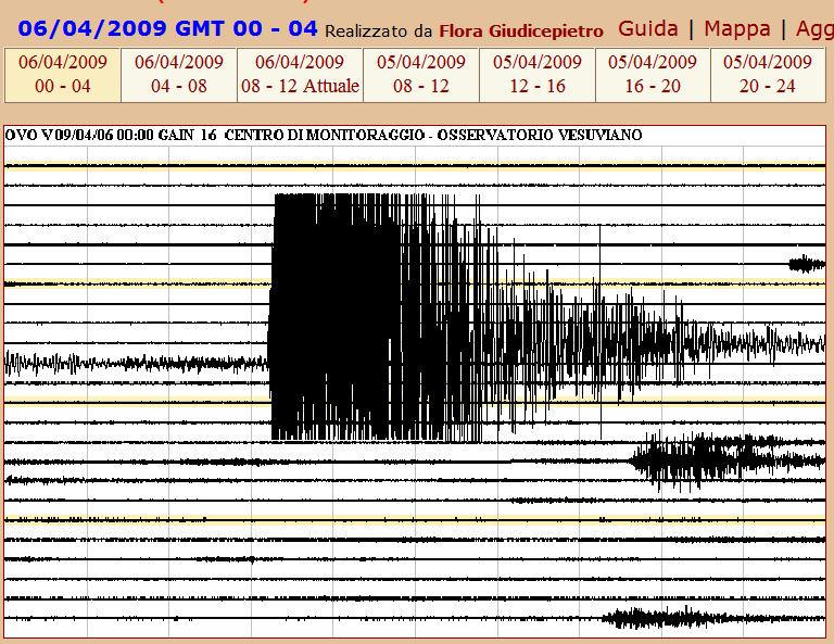
Geophysical Research Abstracts,
Vol. 10, EGU2008-A-10334, 2008
SRef-ID: 1607-7962/gra/EGU2008-A-10334
EGU General Assembly 2008
© Author(s) 2008
Radon precursors to earthquakes: a search for physical
mechanisms
H. Woith (1), G. Martinelli (2), J. Heinicke (3) & H. Surbeck (4)
(1) GeoForschungsZentrum Potsdam, Germany, (2) Servizio Cartografico e
Geologico,
Regione Emilia-Romagna, Bologna, Italy, (3) TU Bergakademie Freiberg, Germany,
(4) Swiss
Center of Hydrogeology, University of Neuchatel, Switzerland (radon@gfz-potsdam.de
/ Fax:
+49 331 2881204)
We investigated a series of publications where radon anomalies were reported to
precede
earthquakes with special emphasis to the proposed physical mechanisms. The
aim of our study is not an in extenso listing of all reported radon anomalies
but rather
an attempt to elaborate certain classes of radon anomalies and their physical
origin. By
far the most popular attempt to relate radon anomalies with earthquakes was –
and still
is – a 1:1 approach, i.e. one radon anomaly is related to one earthquake.
Whereas the
anomaly definition is more or less straightforward, the selection of the
“corresponding”
earthquake is not. In fact, it is the most critical, sometimes arbitrary
procedure.
Other types are 1:n and n:n relations describing one radon anomaly in relation
to the
seismicity of an area or a time segment and a series of radon transients in
relation
to seismicity in time and/or space, respectively. Finally, we discuss 1:0 types
of relations,
i.e. a radon anomaly which is not followed by an earthquake. Needless to say,
that the latter type is rarely published. We will present examples that
non-seismically
originated radon anomalies can be strikingly similar to the “real” thing and
thus the
underlying physical processes might be strikingly similar as well.
E in Thailandia vediamo cosa scrivono al riguardo:
Soil gas radon as an earthquake precursor: some considerations on data
improvement
References and further reading may be available for this article.
To view references and further reading you must purchase this article.
K. Wattananikorna,
M. Kanareea
and S. Wiboolsakea
a Department of Physics, Faculty of Science, Chiang Mai University,
Chiang Mai 50200, Thailand
Received 6 June 1998;
accepted 24 July 1998.
Available online 28 January 1999.
Abstract: A data processing technique based on impulse responses
from multivariable time series was applied to radon data. It was found that soil
gas radon at 50 cm depth was affected more by meteorological parameters than at
100 cm depth. This fact together with the fact that the radon change at the
latter depth was larger when an earthquake occurred, radon measurement at 100 cm
depth was tested as an earthquake precursor. The result showed correlation
between radon anomalies and earthquake events.
Article Outline
-
1. Introduction
-
2. Geology of the study area
-
3. Meteorological and earthquake data collection
-
4. Radon measurement
-
5. Theoretical consideration
-
5.1. Movement of radon in overburden
-
5.2. Radon data processing
-
6. Result and discussion
-
6.1. Improvement of soil gas radon data
-
6.2. Radon data as an earthquake precursor
-
7. Conclusion
- Interessante!!! Non lo sanno neppure loro. Vediamo se anche altri ignorano
la cosa... Ora andiamo in India...
Lascio l'articolo in Inglese perché e' bene conoscere almeno tre lingue
oggigiorno e un poco di sforzo no fa mai male.
COMMUNICATIONS
1288 CURRENT SCIENCE, VOL. 86, NO. 9, 10 MAY 2004
A study of fluctuation in radon concentration behaviour as an earthquake
precursor
Kaushik Majumdar
Electronics and Communication Sciences Unit, Indian Statistical
Institute, 203, B.T. Road, Kolkata 700 108, India
Before, during and after many large earthquakes significant
change in concentration of radon has been
observed in China, Japan and India. To establish this
behaviour as a potential earthquake precursor, it is
important to understand the phenomenon in terms of
geodynamics. Here I propose a geodynamic model to
establish a correlation between precursory radon concentration
fluctuations and an impending earthquake.
The model has been validated by field data collected
from Japan and China. Further investigation with this
model also helps to find a possible explanation for
abnormal variation in the geomagnetic field intensity
observed before, during and after some earthquakes.
LARGE earthquakes (M 5.5 or more) are the most devastating
of all natural calamities to human life and property.
Therefore, scientific research leading to successful prediction
of large earthquakes, sufficiently in advance, has
great significance to mankind. Unfortunately, to this date,
no reliable method for successful earthquake prediction
with precise timing, location and intensity has been developed.
Nevertheless, based on long-time studies, some
earthquake precursors like change in ion concentration in
water, variation in concentration of He, Ne, Ar, Rn and
N2 in the environment of the affected zone, abnormality
of behaviour in some animals, occurrence of milder foreshocks
before a large earthquake, sudden water-level change
in some wells, ground deformation, stress build-up in the
ground rocks (which may in turn alter electric resistance
of the rocks)1, etc. have been identified. But most of these
precursors behave erratically and therefore have been
poorly understood so far and earthquake prediction has
become a controversial issue2,3.
To understand the exact relationship of a precursor
with an impending large earthquake, it is essential to
know the geodynamical reason behind the occurrence of
that precursor. Erratic change in radon concentration has
been observed in many earthquake-prone zones a few
months before, during and after a large earthquake1,4–6.
Such behaviour has been observed in deep wells where
inducement of radon concentration fluctuations from the
environment can virtually be ruled out. Therefore, it is
tempting to consider a sudden erratic fluctuation in radon
concentration, for days on end, particularly in deep wells
in an earthquake-prone zone, as a potential omen for an
impending large earthquake. Here an analysis of the precursory
radon concentration behaviour during the Izu-
Oshima-kinkai earthquake (M 7.0) during 1978 in Japan
will be undertaken, and based on this a geodynamic model
will be proposed, which has been validated by data collected
during some other earthquakes.
Let us try to find an explanation for the erratic fluctuations
in radon concentration recorded in an artesian well
in Izu peninsula of Japan, before, during and after the
14 January 1978 Izu-Oshima-kinkai earthquake (M 7.0,
Figure 1)4.
Most of the rocks in the earth’s crust, as well as soil
and alluvium derived from it, contains uranium. About
99.3% of this uranium7 is the isotope U-238. Decay of an
U-238 atom marks the beginning of a series of 14 decays
that ends at the isotope Pb-206. Rn-222 (half-life 3.82
days, directly derived from Ra-226) is an intermediate
radioactive, inert, odourless, colourless, gaseous daughter
isotope in the decay7 of U-238 to Pb-206. Because of the
short half-life of Rn, it is generally believed that most of
the naturally occurring Rn in the environment comes
from only within a few metres of depth in the earth’s
crust7. The continental crust has an average thickness of
30 km, reaching its highest value of 70 km in the Tibetan
plateau8, and minimum at the spreading plate boundaries.
A standard argument for the variation in dissolved gas
concentration in water wells before, during and after an
earthquake in that zone, is the variation in release of the
gases entrapped in crustal rocks due to pore collapse and/
or crack build-up caused by variation in stress5. Being an
inert gas, radon concentration cannot be varied due to
chemical reaction with other substances exposed due to
crack build-up in the rocks. Normally, its source on the
earth is U-238 in the near-surface crustal rocks, whose
typical concentration level is 1 to 4 parts per million (ppm)7.
To explain the erratic precursory radon concentration
behaviour4 in Figure 1, I propose the following model.
e-mail: kaushik_r@isical.ac.in
RESEARCH COMMUNICATIONS
Figure 1. Precursory radon concentration fluctuations of 1978 Izu-
Oshima-kinkai earthquake observed in an artesian well, 25 km away
from the epicentre. The heavy dotted line shows the average annual
variation calculated from data for eight years. (After Wakita et al.4).
RESEARCH COMMUNICATIONS
CURRENT SCIENCE, VOL. 86, NO. 9, 10 MAY 2004 1289
The pattern of convection beneath the earth’s surface
plate, on which the plate tectonics and therefore earthquakes
depend, remains one of the main unsolved problems
in geophysics9. Because both seismic earth models
and mineral physics studies suggest that any present-day
chemical density heterogeneity in the mantle cannot exceed
1–2%, the mantle is often assumed to be homogeneous
for the purposes of dynamic modelling9. Clearly, this is
only an approximation. The upper mantle, near the subduction
zones, where subducted lithospheres with strong
chemical heterogeneity on the scale of tens of kilometres8
are slowly being recycled back into the mantle, must bear
the signature of this heterogeneity. In fact, chemical
segregation is favoured over homogenization by kinematic
mixing8.
In laboratory experiments, under much more simplified
conditions compared to the actual mantle, ‘doming’ regimes
have been observed at a layer of viscosity stratification in
a thermochemical flow model9. The Rayleigh numbers of
the experiments are comparable to those of the actual
mantle flow. Hot plumes come out from a small neighbouring
area centering the uppermost point of the dome.
In a recent study, four high-viscosity stratification layers
in the mantle have been identified, the uppermost being
only 220 km deep10. Chemical heterogeneity near a subduction
zone, coupled with this viscosity stratification,
should also give rise to smaller (only of the order of a
few thousand cubic km), shortlived blobs (existing only
for a few tens of years before being mixed-up in the
mantle), unlike the megablobs in existence for hundreds
of million of years, as inferred by Davaille9. Hot, cylindrical,
axisymmetric plumes of diameter only from a few
hundred metres to a few kilometres will reach up to just
below the plates. There is a region of upper mantle, 50 to
150 km deep, with low viscosity10 and low seismic velocity8
(i.e. with low density) over which plates glide, like
rafts floating on sea. Hot-plume injection in this region
near a subduction zone will expedite plate motion, by
reducing viscosity and/or increasing negative buoyancy
(by density reduction), which may lead to the advancement
of an earthquake. In this regard, it is interesting to
note the excellent correlation observed between seismic
activity of an earthquake-prone zone with artificial injection
of water in the rocks1, although the two mechanisms
and effects are completely different.
Studies carried out10, clearly indicate that the flow inside
the mantle is turbulent, in the sense that (i) the
velocity field is random and (ii) vortices occur chaotically.
Turbulent flow and temperature variations in the
upper mantle may occasionally increase the pressure
inside the blob, leading to a sudden increase in plume
discharge from it. This, in turn, will increase the plate
motion sometimes (but not always) leading to an earthquake.
Alternatively, the conduit through which the plume
is upwelling may get choked for sometime, leading to a
pressure build-up inside the blob. When the pressure
level becomes sufficiently high the conduit may burst,
much like a blocked pressure cooker valve, ejecting
greater amount of plumes than usual for sometime, till
the pressure level inside the blob returns to normal. This
process may expedite the plate motion more than it has
initially slowed down depending on the duration of
choking and the magnitude of the upwelled magma after
the blast.
To explain the precursory erratic radon concentration
behaviour of Izu-Oshima-kinkai earthquake (Figure 1),
let us note that the high annual average radon concentration
cannot be due to a source from near the surface of
the earth, but rather from much deeper underground. It is
actually coming out of the Moho through a conduit
across the plate. The Moho in this region got its supply
(steady at least for several years) of U-238 from a blob
just underneath, through upwelling plumes. Just a few
months before the 14 January 1978 event, the magma
upwelling conduit above the blob got choked-up, leading
to an intermittent release of smaller-than-usual amount of
uranium. (The uranium concentration is diluted fast through
mixing in the low viscosity and low density region,
where the velocity of ejection is much higher than the
usual convection speed in that layer.) The average concentration
of U-238 in the interior of the earth8 is 30.8 ×
10–9 kg/kg and that at the uranium ore7 is 10–3 kg/kg, as
characterized by sudden step-like lowering in the rate of
radon emission in Figure1. When the burst occurred, it
cleared the block at the magma upwelling conduit leading
to a greater-than-usual uranium supply at the Moho just
above, which in turn increased the radon emission rate
just before and after the 14 January event, as shown in
Figure 1. The hypothesis is further bolstered by the data
presented in Figure 2 in conjunction with the abovementioned
radon emission rate (see Figure 2 a). In Figure
2 b, water-temperature variation in a 500 m well, at
an epicentral distance of 30 km, has been recorded. In
Figure 2 c and d water-level variation at the well of
(Figure 2 b) and the ground strain variation (at a borehole
strain-meter placed at an epicentral distance of 50 km)
have respectively been recorded. From the data of Figure
2, it is apparent that the water in the well (Figure 2 b) is
directly being heated by hot gas emanating from the
plume under the plate and reaching the well by diffusion
through small cracks across the plate (unfortunately, no
chemical analysis data of the well-water at that time is
available to further confirm or reject this assumption). As
the plate slowly subducts, the ground strain is relaxed
leading to crack enlargement, which decreases the water
level in the well (by 0.3 m) by consuming some of it. But
since the plume has ceased to upwell due to temporary
choking of the plume conduit over the blob in the upper
asthenosphere region8, the water temperature falls instead
of increasing even after enlargement of the cracks. This
is compatible with a similar fall in the radon emission
rate level at the well (Figures 1 and 2 b).
The subsequent
RESEARCH COMMUNICATIONS
1290 CURRENT SCIENCE, VOL. 86, NO. 9, 10 MAY 2004
rise in radon emission rate level (Figure 2 a) and watertemperature
increase (Figure 2 b) are also compatible. It
is worthwhile to note that during observation of radon
concentration in the well of Figure 1 from May 1977 to
August 1986, no significant change was observed due to
other earthquakes of magnitude greater than M 5 within
an epicentral distance of 100 km and greater than M 6.5
within 600 km4.
A simple mathematical model of elliptic spreading of
hot magma (for clue see Figure 1 b of Manga11), in the
Moho, ejected through the plume conduit on top of a blob
is being proposed. According to this model, the twodimensional
magma flow in the Moho is turbulent at any
point of time. According to some opinion, turbulent flows
cannot be modelled by the Navier–Stokes equations12,13.
Here I propose the following set of equations for modelling
the two-dimensional magma spreading through the
Moho. (Equations (1) and (2) represent a general form of
flow in a plane. By choosing the values of ni, Ai, mi and
the form of the functions fi, any flow in a plane can be
modelled by eqs (1) and (2), as shown here in case of an
elliptical flow.)
( , , )
1( 1 2 ) 1( 1 2 ) 1 , , , , e 1 1 1 2 m f x x t u x x t v x x t A - = + , (1)
.
( , , )
2 ( 1 2 ) 2 ( 1 2 ) 2
u x , x , t = v x , x , t + A e-m2 f2 x1 x2 t (2)
ui is the total velocity component along xi, vi is the linear
velocity along xi, Ai emifi(xi,x2,t) is the curvilinear (spiral)
component of velocity along xi, for i = 1, 2. Ai and mi
are constant numbers whose values lie in some closed,
bounded intervals of the real line. (The absolute value of
mi is an increasing function of Rayleigh number and
determines the angular shape of curving, Ai determines
the radius of the curving), fi is a function giving the
angular span of curving. A1 and A2 are of the order of tens
of kilometres. Moreover, if the flow is approximately
elliptical, then we should take
log(sin )
1
1
f1 t m = and
log(cos )
2
1
f2 m t = ,
where t is of the order of years and therefore sint and cost
can be taken as positive in a few months to few years
range. Since here I am concerned with the curvilinear
spreading of flow only, keeping the centre of propagation
(the hole of plume ejection) fixed, v1 = v2 = 0.
Geochemical heterogeneity within the upper mantle is
not limited to the subduction zones alone. Due to existence
of diverse isotopic suits throughout the upper
mantle, the upper mantle has been modelled like a ‘plum
pudding’14. So blobs can also form below, deeper inside
the plate. Ejection of plumes from such blobs may affect
the intraplate stress build-up, expediting an intraplate
earthquake.
In a two-layer mantle convection model, the concentration
of radiogenic heat sources (U-238, U-235, Th-232
and K-40) in the lower mantle is only about 1.5% of the
average heat-source concentration in the entire mantle8.
In a more detailed model, the upper mantle itself is subdivided,
according to viscosity stratification, into two
zones separated by a high-viscosity layer at 220 km
depth10. The density variation is the highest in the whole
mantle above this layer10, possibly forming the continental
and the oceanic crusts at the surface, like accumulation
of cream over boiled milk after cooling. Mantle flow
through the high viscosity barriers (at least four)10 is
Figure 2. Precursory changes of the 1978 Izu-Oshima-kinkai earthquake.
a, Radon concentration change observed at the well of Figure 1.
b, Water-temperature variation observed at a 500 m well (epicentral
distance 30 km). c, Water-level variation at the well of (b). d, Strain
change measured by a borehole strainmeter at the tip of the peninsula
(distance 50 km). After Wakita et al.4.
a
b
c
d
RESEARCH COMMUNICATIONS
CURRENT SCIENCE, VOL. 86, NO. 9, 10 MAY 2004 1291
maintained through upwelling of plumes in a smaller
scale, compared to the ones in Hawaii, which gradually
depletes the lower parts of the mantle of radiogenic heat
producing materials and enriches the upper parts of the
mantle with their deposit. This process becomes the
richest in radiogenic substances through the uppermost
high-viscosity layer at 220 km depth. The spike-like fluctuation
in the precursory radon concentration behaviour
before several earthquakes of intensity M 5.5 or more, as
recorded in Guza station (located at the intersection of
three major fault systems)4 in China (Figure 3), is
directly related to this phenomenon. The smaller plume
conduits, where plume strength varies in time and possibly
deformed by other motions in the flow, often tend to
get choked-up. Due to radiogenic heating inside the blob,
the pressure keeps building up. When the pressure becomes
sufficiently high, the choke in the conduit is blown
up, releasing a sudden spurt of U-238-rich plume for
some-time before being choked-up again. This may affect
the strain build-up in the plate directly above by expediting
the plate motion, sometimes (but not always)
leading to an intraplate earthquake. Radon, produced by
U-238 decay, might be reaching the station through some
cracks across the plate and after the plume conduit chokes
up, the uranium concentration below the plate is diluted
fast through rapid mixing in the low-viscosity and lowdensity
region.
The simulation given in Figure 4 will help analyse the
precursory change in geomagnetic field intensity during
some moderate-to-large earthquakes in China and Mongolia
(Figure 5).
The propagation of hot magma as shown in Figure 4, is
in general turbulent, due to numerous collisions with the
subsolidus rock. But if the radioisotope-rich magma at
some portion gets an average angular velocity, as shown
in Figure 4, then the emitted a, b and g rays due to
radioactive decay ionize some of the neighbouring materials
and release free electrons. The circulation of free
electron-rich magma in a path indicated by arrows in
Figure 4, will produce a magnetic field. According to its
orientation, it may increase or decrease the geomagnetic
field intensity as experienced on the surface of the earth.
Magma upwelling below a plate near the boundary
may help plate subsistence due to negative buoyancy (upwelled
magma is hotter and therefore less dense than the
surrounding). This may expedite an interplate strike-slip
earthquake, like the one that occurred on 12 June 1897 in
Assam, India (M 8.1)15. Radon concentration fluctuation
monitoring has been going on for about two decades in
the Himalayan region also6,16. Here too, the correlation
between erratic fluctuations in radon concentration and
seismic activity is clear6,16. It has been demonstrated that
Figure 3. Spike-like changes in radon concentration observed at
Guza station, Sichuan Province, China before several earthquakes of
magnitude M 5.5 or more, within an epicentral distance of 320 km.
After Wakita et al.4.
Figure 4. Magma propagation below the plate after upwelling
through an axisymmetric plume at the centre (diameter 2 km). In
reality, the upwelled magma will collide with the subsolidus rock in the
Moho and the velocity vector will be random at each point. A more
complicated calculation of eqs (1) and (2) at a finer resolution will give
a more realistic simulation. But even the present simple simulation will
help explain phenomena like precursory change in geomagnetic field
intensity4. If the radioisotope-rich magma in certain regions gets an
average angular velocity as indicated by the arrows, it will affect the
geomagnetic field intensity.
RESEARCH COMMUNICATIONS
1292 CURRENT SCIENCE, VOL. 86, NO. 9, 10 MAY 2004
even in case of small earthquakes (M 4.5 or less), erratic
fluctuations in radon concentration is clearly observable
before, during and after an earthquake16. Radon concentration
fluctuation data collected from Chamba station (in
Himachal Pradesh, India) during March 1995 have been
presented in time series form (see figure 3, Virk et al.6).
An earthquake of M 5.1 occurred in Chamba on 24 March
1995. Here too, several days before the quake, radon
concentration level went down (possibly because of choking
as described above) and then suddenly shot up
abnormally (because of the sudden burst of the choked
conduit) a few days before the earthquake. Right at the
time of the quake, it reached almost the usual level. But
the earlier events had already expedited the plate motion,
leading to the 24 March earthquake, or at least some
advancement of it.
Validating an earthquake precursor through an acceptable
geodynamic modelling and accounting for its occurrence
is a challenging task. Earthquakes are seen as consequences
of plate tectonics. Plate motions are controlled
by the complex dynamics of mantle flows, which depends
on the thermal states and chemical composition of the
mantle. Upwelling of hot plumes and downwelling of
colder, denser materials keep running the cycles of vertical
mantle flow over geologic time. Therefore, it is only natural
to expect that plume upwelling and propagation below
the plates may have significant effects on the seismic
activities. Based on the findings of some recent research9,10,
here a model has been proposed for upwelling and spreading
of radioisotope-rich magma below the plates, which
leaves its signature in the erratic radon concentration
fluctuations, as observed before, during and after some
earthquakes in China, Japan and India. With this model,
the geomagnetic field intensity change as a precursor to
some earthquakes can also be explained. Based on the
validity of the model, radon concentration and geomagnetic
field intensity variation give a direct measure of the
velocity field and chemical composition of magma
upwelling and propagation below the plate, from which
the prospect of an intermediate-term prediction of an
impending large earthquake can sometimes be improved.
This should be viewed as a complementary and not
competitive effort for earthquake prediction in addition to
the existing ones like the measurement of rupture
propagation3,17. Further testing of this model with more
diverse datasets is needed.
1. The Cambridge Encyclopaedia of Earth Sciences, Cambridge
University Press, Cambridge, 1981.
2. Geller, R. J., Shake-up for earthquake prediction. Nature, 1991,
352, 275–276, Nature, 353, 611–612.
3. Vidale, J. E., Do big and little earthquakes start differently? Science,
1996, 271, pp. 953–954.
4. Wakita, H., Nakamura, Y. and Sano, Y., Short-term and intermediateterm
geochemical precursors. In Intermediate-Term Earthquake
Prediction (eds Stuart, W. D. and Aki, K.), Birkhauser, Basel,
1988, pp. 267–278.
5. Donald, T., Geochemical precursors to seismic activity. In Intermediate-
Term Earthquake Prediction (eds Stuart, W. D. and Aki,
K.), Birkhauser, Basel, 1988, pp. 241–266.
6. Virk, H. S., Walia, V. and Sharma, A. K., Radon precursory signals
of Chamba earthquake. Curr. Sci., 1995, 69, pp. 452–454.
7. http://www.azgs.az.gov/RADONDTE.htm, Spencer, J. E., Radon
gas – a geologic hazard in Arizona. In Arizona Geological Survey:
Down-to-Earth Series 2, 1992.
8. Schubert, G., Turcotte, D. L. and Olson, P., Mantle Convection in
the Earth and Planets, Cambridge University Press, Cambridge,
2001.
9. Davaille, A., Simultaneous generation of hotspots and super-wells
by convection in heterogeneous planetary mantle. Nature, 1999,
402, 756–760.
10. Forte, A. M. and Mitrovica, J. X., Deep-mantle high-viscosity
flow and thermochemical structure inferred from seismic and geodynamic
data. Nature, 2001, 410, 1049–1056.
11. Manga, M., Shaken, but not stirred. Nature, 2001, 410, 1041–
1043.
12. Ladyzhenskaya, O. A., The Mathematical Theory of Viscous Incompressible
Flow, Gordon and Breach, New York, 1969.
13. Hardy, J. and Pomeau, Y., Microscopic model for viscous flow in
two dimensions. Phys. Rev. A, 1977, 16, 720–726.
14. Batiza, R., Inverse relationship between Sr isotope diversity and
rate of oceanic volcanism has implications for mantle heterogeneity.
Nature, 1984, 309, 440–441.
15. Bilham, R. and England, P., Plateau ‘popup’ in the great 1897
Assam earthquake. Nature, 2001, 410, 806–809.
16. Virk, H. S., Sharma, A. K. and Walia, V., Correlation of alphalogger
radon data with microseismicity in N-W Himalaya. Curr.
Sci., 1997, 72, 656–663.
17. Kasahara, K., Earthquake Mechanics, Cambridge University Press,
Cambridge, 1981.
18. Hart, S. R., A large-scale isotope anomaly in the southern hemisphere
mantle. Nature, 1984, 309, 753–757.
19. van der Hilst, R. D. and Karason, H., Compositional heterogeneity
in the bottom 1000 kilometers of Earth’s mantle: Toward a hybrid
convection model. Science, 1999, 283, 1885–1888.
ACKNOWLEDGEMENTS. During this research I was supported by
a Senior Research Fellowship of the Indian Statistical Institute and
received some technical help from Mr Subhashis Mitra. Helpful suggestions
made by the anonymous reviewers are acknowledged.
Received 15 July 2003; revised accepted 24 February 2004
Figure 5. Geomagnetic field intensity change observed in Beijing,
during the earthquakes in Holinkoerh, Inner Mongolia (6 April, M 6.3),
Tacheng (22 April, M 4.4) and Tangshan (28 July, M 7.8 and 7.1), both
in China. Taken from Wakita et al.4 after editing out the portions which
are not relevant to this study.
E ora torniamo in Italia.... ma siamo proprio sicuri che non se ne sapeva
nulla?
Tracking precursors and degassing by radon monitoring during major
eruptions at Stromboli Volcano (Aeolian Islands, Italy)
Tracking precursors and degassing by radon monitoring during major eruptions at
Stromboli Volcano (Aeolian Islands, Italy)
C. Cigolini DSMP, Università di Torino, Turin, Italy
G. Gervino DFS, Università di Torino, Turin, Italy
R. Bonetti IGGA, Università di Milano, Milan, Italy
F. Conte DSMP, Università di Torino, Turin, Italy
M. Laiolo DSMP, Università di Torino, Turin, Italy
D. Coppola DSMP, Università di Torino, Turin, Italy
A. Manzoni IGGA, Università di Milano, Milan, Italy
Ma sono tutti ricercatori Italiani che scrivono in Inglese!!!
Come mai?
We monitored radon anomalies before, during and after the recent paroxysmal
eruptions of Stromboli. Major eruptive events are preceded by relative minima in
radon emissions at stations located at the base of the cone, whereas three of
the summit stations reached peak values (∼20,000 Bq/m3 or
higher) 12 to 14 days before major eruptions, and are nearly coeval with earth
tides. Radon emissions at/or above such high threshold values are proposed to
result from the dynamic response of the fracture network due to degassing
processes associated with magma ascent. Relative minima recorded at the base of
the cone are related to fractures' self-sealing within the hydrothermal system,
eventually coupled with the atmospheric stack-effect. The coexistence of the
above anomalies is interpreted as the first precursory signals to major eruptive
events.
Received 2 February 2005; accepted
19 May 2005; published 24 June
2005.
Citation:
Cigolini, C., G. Gervino, R. Bonetti, F. Conte,
M. Laiolo, D. Coppola, and A. Manzoni (2005),
Tracking precursors and degassing by radon monitoring during
major eruptions at Stromboli Volcano (Aeolian Islands, Italy),
Geophys. Res. Lett.,
32, L12308, doi:10.1029/2005GL022606.
Questi posso prevedere addirittura le urruzioni vulcaniche con 12 / 14 giorni
di anticipo!!! Viva i Profeti del Vulcano !!!
The Smithsonian/NASA Astrophysics Data System
Natural Radioactive Characterization by Gamma Ray Mapping in
Relation with Radon-222, Radium-226 Contents in the
Atmosphere, Dripping Groundwater and Mineral in a Dead-end Horizontal Tunnel
American Geophysical Union, Fall Meeting 2004, abstract #H21E-1059
The concentration of radon-222 has been monitored since
1995 in the atmosphere of a 2 m transverse dimension, 128 m long, dead-end
horizontal tunnel located in the French Alps, at an altitude of 1600 m. The
total volume of the tunnel is about 496 m3 with an estimated total
wall surface area of 1041 m2. Most of the time, the
radon concentration is stable, with an average value ranging from 200 Bq
m-3 near the entrance to about 1000 Bq m-3 in the most
confined section, and with an equilibrium factor F between radon
and its short-lived decay products varying from 0.61 to 0.78. However,
radon bursts are repeatedly observed, with amplitudes
reaching up to 36 x 103 Bq m-3 and durations varying from
one to several weeks, with similar spatial variations along the tunnel as the
background concentration. These spatial variations are qualitatively interpreted
in terms of natural ventilation. To understand the source term, we realised a
comprehensive 3D map of total gamma emission of rock on all surfaces of the
tunnel, i.e., floor, wall and roof, representing 700 measurements points with a
section of eight points by two-meter steps along the tunnel. Dose rate varies
from 100 to 350 nSv h-1 and reveals two major contrasted geological
structures, correlated with the radon-222 profile in the
air along the tunnel (230 Bq m-3 at the entrance to 770 Bq m-3
at the end, measured during a period of background radon
level), and with other profiles measured in previous work. In addition, a
correlation is evidenced with the radon-222 contents in
dripping groundwater and with the radon
precursors - i.e., the daughters of uranium-238 (radium-226, for example)
- content in rocks. The radon and radium contents in
water and rocks, and the study of flow rate of the dripping groundwater are in
direct relation with the mechanism of radon gas transport
by water in porous media. By interpreting all available measurements, it is now
possible to model the time variation of radon-222 in the
tunnel, and to constrain the origin of the radon peaks
generated in the gallery. The bursts result from transient
radon exhalation upsurges at the tunnel wall, that
could be due to meteorological effects, or possibly
to combined hydrological and mechanical forcing
associated with the water level variations of the nearby Roselend reservoir lake.
Mechanical Forcing suona un po come stress sismico non e' vero? Ma ora
andiamo in Antartide....
The peculiarities of cross-correlation between two secondary
precursors - radon and magnetic field variations, induced by tectonic activity
( Ma daiii... )
(Submitted on 29 May 2006)
Abstract: A model of precursor manifestation
mechanisms, stimulated by tectonic activity and some peculiarities of observer
strategy, whose main task is the effective measurement of precursors in the
spatial area of their occurrence on the Earth's daylight, are considered. In
particular, the applicability of Dobrovolsky's approximation is analyzed, when
an unperturbed medium (characterized by the simple shear state) and the area of
tectonic activity (local inhomogeneity caused by the change only of shear
modulus) are linearly elastic, and perturbation, in particular, surface
displacement is calculated as a difference of the solutions of two independent
static problems of the theory of elasticity with the same boundary condition on
the surface. Within the framework of this approximation a formula for the
spatial distribution (of first component) of magnetic field variations caused by
piezomagnetic effect in the case of perturbed regular medium, which is in simple
shear state is derived. Cogent arguments in favor of linear dependence between
the radon spatial distribution and conditional deformation are obtained.
Changes in magnetic field strength
and radon concentrations were
measured along a tectonomagnetic profile of the total length of 11 km in
the surroundings of the "Academician Vernadsky" Station on the
Antarctic Peninsula (W 64 16', S 65 15'). Results
showed a positive correlation between the annual surface radon concentration and
annual changes of magnetic field relative to a base point, and also the good
coincidence with theoretical calculation.
Allora vediamo se in casa nostra nonlo
sapeva proprio nessuno... o e' il solito segreto di pulcinella...
A. Riggio, S. Sancin, G. F. Gentile, P.
Zennaro e R. Belletti
Istituto
Nazionale di Oceanografia e di Geofisica Sperimentale, Trieste
MISURE DI RADON
IN FRIULI E CONFRONTO CON LA SISMICITÀ
Riassunto.
Scopo del lavoro è quello di
contribuire alla conoscenza dello stato di stress presente nelle strutture,
verificando eventuali correlazioni tra emissione di radon e attività sismica. A
tal fine, nel 1995, è stata installata una stazione per il rilevamento del gas
radon in Friuli, in funzione continuativamente dal 1996 a meno di alcune piccole
interruzioni dovute a cause tecniche. Nel presente lavoro è considerato il
periodo 1996-1997 per uniformità di dati. Contemporaneamente sono stati
controllati i parametri meteorologici e l'andamento della falda freatica. È
stata riscontrata una scarsa dipendenza della concentrazione di radon dai
parametri meteorologici, ma temperatura e radon hanno in comune le variazioni
giornaliere e le variazioni stagionali. Tramite la "crosscorrelazione del
segnale giorno per giorno", è stato messo in evidenza che le possibili
"anomalie" sono costituite da variazioni nell'andamento giornaliero del gas
radon. L'accostamento degli eventi sismici, verificatisi durante il periodo
preso in esame, mostra i possibili legami tra variazione di radon e terremoti
più forti. Le variazioni più significative sono state accompagnate da variazioni
del livello di falda non giustificate dalla pluviometria.L'anomalia più
evidente, anche nella semplice rappresentazione della concentrazione del gas
radon, è quella presente durante il periodo gennaio-marzo 1996. In questo
periodo si è verificata la serie sismica di Claut costituita da tre terremoti
principali che, con 3,7, 4,0 e 4,3 di magnitudo, sono stati i più forti con
epicentro entro il territorio regionale, da gennaio 1996 a dicembre 1997.
RADON
MEASUREMENTS IN FRIULI AND COMPARISON WITH THE SEISMICITY
Abstract.
The purpose of this
work is to contribute to knowledge of the stress status of the structures by the
control of the possible correlation between radon emission and the seismic
activity.For this end, on 1995, a radon survey station has been set up in Friuli
and since 1996 it is recording continuously. In this work has been considered
the period 1996-1997 for homogeneity of the radon data. At the same time have
been controlled meteorological parameters and the groundwater level. The radon
concentration results connected with the meteorological parameters in a quite
weak way, but temperature and radon show the same behaviour and the same
seasonal variation.Through the "day by day croscorrelation of the signal" has
been pointed out that the "anomaly" consists mainly of a daily behaviour
variation of the radon concentration. The coupling of the seismic events have
showed the correlation between the radon variation and the strongest
earthquakes. During more important radon variations, also the groundwater level
changes without any rain justification.The clearest anomaly, in the same radon
concentration representation too, has been noticed during the period
January-March 1996. In this period happened the Claut seismic series constituted
by three main earthquakes that with magnitude 3.7, 4.0 and 4.3, have been the
strongest verified over whole region since 1996 January to 1997 December.
INTRODUZIONE
La
Previsione dei terremoti, intendendo con questa, quando, dove e con quale
energia si verificherà un evento sismico, come sanno bene tutti gli "addetti ai
lavori", rimane ancora un'aspirazione per tutti (Wyss, 1991).
I tentativi
portati avanti in passato sia dalle varie scuole (russa, cinese, greca, ecc.)
che da dilettanti, hanno trovato spesso l'opposizione della comunità
scientifica, perché ritenuti non significativi. Il nocciolo del problema è
capire come gli stress che possono precedere un terremoto o provocare lenti
movimenti, si propaghino nel sottosuolo e come le strutture reagiscano ad essi.
Questo comporta l'analisi delle strutture dal punto di vista dinamico attraverso
lo studio delle variazioni nel tempo dei parametri fisici sensibili agli stress
(Ren et al., 1984; Kissin et al., 1996; Cosentino et al., 1976; Riggio e Sancin,
1986; Riggio et al., 1987). Tra questi parametri, la concentrazione di radon ha
la caratteristica di poter essere rilevata con un costo relativamente basso e di
essere molto sensibile alle variazioni di stress anche profondo e proveniente da
strutture più lontane. Il radon si diffonde attraverso le rocce e si disperde
nel suolo e nell'acqua in cui ha buona solubilità (Dongarrà e Martinelli, 1995;
Martinelli, 1992; Martinelli, 1993).
La misura del
radon è utilizzata per scopi tettonici (per individuare faglie sepolte,
controllare quelle attive dopo disastrosi eventi sismici, etc.) (Facchini et
al., 1995), per individuare dei percorsi idrici e per scopi ambientali (radon
indoor, individuazione delle perdite di biogas nelle discariche, inquinamenti da
idrocarburi, ecc.).
Le fratture che
si formano prima di un terremoto, secondo il modello della dilatanza (Birchard e
Libby, 1980) incrementano la diffusione del fluido nei pori, quindi modificano
la resistenza e la pressione della roccia cosicché il flusso del radon viene in
qualche modo modulato dagli stress. Queste variazioni sono considerate
significativi precursori del terremoto (Riggio e Sancin, 1995).
Le prime
applicazioni di questo tipo di misure furono fatte in Unione Sovietica, e i
primi risultati positivi si ebbero in coincidenza del terremoto del 1966 a
Tashkent (Mogi, 1985). Il graduale incremento nei valori di concentrazione di
radon iniziò già sei anni prima del terremoto e si stabilizzò alcuni mesi prima.
Le anomalie di radon si presentano in forme differenti: con incrementi o
decrementi, con variazioni lente o rapide tipo "spike" (Friedman et al., 1988;
Heinicke et al., 1995). Attualmente misure continue di radon vengono eseguite in
Cina, Giappone, Stati Uniti e altri paesi. Negli Stati Uniti ebbero occasione di
notare anomalie di radon in corrispondenza di quattro sismi con magnitudo tra
4,2 e 4,7.
Anche in Italia
dall'inizio degli anni '90 si sono sviluppati gli studi di monitoraggio della
geochimica dei fluidi miranti ad ottenere le variazioni dei vari parametri, sia
nello spazio che nel tempo (Calcara e Quattrocchi, 1993a, 1993b; Carapezza et
al., 1980; Dall'Aglio, 1992).
IL
PROCESSO FISICO
La
misura della concentrazione di radon è eseguita più frequentemente in acqua, (Friedmann
e Hernegger, 1978; Heinecke et al., 1995), ma non mancano rilevamenti in suolo
(Friedman et al., 1988; Sabbarese et al., 1993). Nonostante il radon abbia un
tempo di dimezzamento di soli 3,5 giorni (Montagner, 1994), sfruttando le
correnti ascensionali di altri gas riesce per convezione a raggiungere la
superficie anche da profondità di vari chilometri. Le variazioni di radon
possono, quindi, essere causate da terremoti con epicentro distante anche
diversi chilometri ma con energia sufficiente. La formula empirica (Hauksson and
Goddard, 1981):
M = 2,4 log10
(D) - 0,43 (1)
definisce
la magnitudo minima M richiesta per ottenere un'anomalia di radon ad una
distanza D espressa in chilometri. Indicativamente un terremoto di magnitudo 4,0
può essere preceduto da un'anomalia di radon fino ad una distanza di 70 km.
Questo valore è interessante in quanto dell'ordine delle massime distanze dei
confini regionali da Cazzaso, sito di rilevamento del radon.
LINEAMENTI
SISMOTETTONICI
Nel 1995 è stata
realizzata una stazione per il rilevamento del gas radon in Friuli, in località
Cazzaso nel comune di Tolmezzo. Nei primi mesi il suo funzionamento è stato
saltuario, e dal 1996 è in funzione quasi continuativamente.
La zona fa parte
dell'area Carnico-Friulana caratterizzata da accavallamenti tagliati da faglie
subverticali a direzione N-S e da altre a direzione dinarica, tutte con attività
spesso trascorrente. L'insieme costituisce, unitamente all'antistante pianura
veneto-friulana, la Catena sudalpina orientale (Bernardis et al., 1996; Slejko
et al., 1987).
L'ubicazione
della stazione per il rilevamento del gas radon è riportata in Fig. 1 dove è
riprodotto anche lo schema tettonico. La zona si trova immediatamente a nord di
quella con la più alta attività sismica che comprende anche l'evento del 1976 di
magnitudo 6,5 (Riggio, Gentile, 1984). In accordo allo schema riportato,
l'abitato di Cazzaso si trova in prossimità della linea Alto Tagliamento e di
una faglia subverticale con direzione Dinarica con attività spesso trascorrente.
Il paese è,
oltretutto, interessato da un evidente dissesto franoso che interessa la zona
delle pendici del monte Diverdalce, la cui nicchia è ben visibile anche da
lontano. La frana sembra avere avuto origine nel novembre 1851 a seguito di un
periodo d'intense piogge. Nel 1898 il movimento franoso causò la distruzione di
alcuni edifici e l'intero paese sarebbe scivolato di circa trenta metri verso
valle.
Storicamente in
questa zona avvennero terremoti disastrosi come quelli di Tolmezzo del 20
ottobre 1788 (Gentile et al., 1984) e del 27 marzo 1928 dell'VIII-IX grado della
scala MCS (Mercalli-Cancani-Sieberg). Poco più ad ovest, il terremoto di Raveo
nel 1700 ebbe un'intensità del X grado MCS ma i suoi effetti furono rilevanti in
un'area molto limitata. Più recentemente, i terremoti che sono avvenuti il 3
febbraio 1949 a Paularo e il 26 aprile 1959 ad Arta, rispettivamente a circa 17
km e a 7 km di distanza da Cazzaso, hanno avuto un'intensità epicentrale dell'VIII
grado MCS.
La sismicità
attuale della zona è costituita da terremoti con magnitudo intorno al 3,0 ed
epicentri tra Tolmezzo, Cazzaso e Villa Santina.
DESCRIZIONE
DELLA STRUMENTAZIONE
La
stazione di rilevamento del gas radon è costituita da un rilevatore denominato
Prassi mod.55 con cella a scintillazione, predisposto sia per la misura continua
che campionata. Il rilevatore è costituito da una camera rivestita internamente
di solfuro di zinco attivato argento. Il volume di questa cella è di 2
litri ed è
accoppiato ad un fotomoltiplicatore a bassa deriva. Lo strumento misura i
conteggi in un tempo prefissato in modo ripetitivo. La concentrazione di gas
radon in Bq/m3 o pCi/l
è calcolata dai conteggi misurati. La larga capacità di memoria permette di
memorizzare fino a 6500 misure. Lo strumento è stato installato all'imboccatura
di un pozzo profondo 40,50 metri con un livello dell'acqua, dal piano di
campagna, di circa 17,5 metri (Fig. 2). La stratigrafia relativa ai primi metri
dal piano di campagna è un'alternarsi di limi sabbiosi-argillosi e ghiaie sino
alla profondità di circa 17 metri, dove iniziano argille più dure, seguono
sabbie, poi siltiti marnose con venature di calcite.
Fig. SEQ Fig. \* ARABIC 1
- Ubicazione della stazione di rilevamento del gas radon e schema
tettonico del Friuli Occidentale da Bernardis et al., (1996).
L'aria viene
aspirata, tramite una sonda flessibile, dal pozzo alla profondità di circa 7
metri dal piano di campagna e a circa 6 metri dalla superficie dell'acqua.
L'intervallo di campionamento è stato fissato in tre ore e 30 minuti,
dall'inizio delle registrazioni sino al 27 maggio 1996, in quattro ore, dal 27
maggio al 17 giugno 1997 e in tre ore, dal 17 giugno in poi. Questi cambiamenti
si sono resi necessari per poter correlare la concentrazione del radon con le
misure meteorologiche che hanno campionamento orario. Lo strumento è stato
protetto, dagli effetti meteorologici, inserendolo in un contenitore in
plexiglas con coperchio a chiusura stagna e alloggiando il tutto in un
armadietto in alluminio con barre di rinforzo e chiusura con lucchetto.
L'alimentazione è realizzata tramite batterie ricaricate con due pannelli solari
e regolatore di carica.
Attualmente,
circa ogni mese viene fatto il recupero dei dati in loco tramite un PC
portatile, ma sarebbe possibile anche trasmetterli direttamente nella sede
dell'elaborazione.
La Regione Friuli-Venezia Giulia,
negli anni 1995-1997 ha stipulato una convenzione con l'OGS al fine di valutare
l'evoluzione del fenomeno franoso. La zona era, quindi, contemporaneamente
attrezzata con pozzi dotati di piezometri e inclinometri tarati per i movimenti
superficiali delle frane, nonché di termometro per la temperatura dell'acqua e
dell'aria, di pluviometro e di barometro.
Fig. SEQ Fig. \* ARABIC 2
- Stazione di rilevamento del gas radon.
ANALISI DEI DATI
Scopo del lavoro
è quello di contribuire alla conoscenza dello stato di stress presente nella
struttura. A tal fine si è proceduto a verificare la presenza di una quantità
sufficiente di radon, la sensibilità della concentrazione di radon alle
variazioni di stress e infine se, in qualche modo, la presenza dello stress
viene confermata da terremoti.
Dal momento che
durante il 1998 è stata apportata una modifica al sistema di rilevamento, per
uniformità di dati è stato considerato il periodo 1996-1997.
La conoscenza dei
parametri meteorologici ha permesso una migliore valutazione dei dati radon, e
di constatare, che con il sistema d'acquisizione usato, le influenze ambientali
sono modeste. Solamente in caso di piogge intense, che possono penetrare
all'interno del pozzo, si possono avere variazioni indotte anche notevoli (in
due anni si è verificato un solo caso, con 40 mm di pioggia in un giorno).
I dati
sismometrici sono quelli registrati dalla Rete Sismometrica del Friuli
Venezia-Giulia, gestita dal CRS (Centro Ricerche Sismologiche) dell'OGS di
Trieste, dalla stazione Broad Band di Trieste, gestita dall'OGS e
dall'Università di Trieste e dal catalogo USGS. I terremoti presi in esame sono
tutti quelli con magnitudo maggiore o uguale a 2,0 (valore minimo per poter
considerare completo il catalogo), e che soddisfano l'equazione (1). Si tratta
in tutto di 95 terremoti, di cui 88 localizzati entro il territorio regionale
(Fig. 3).
Fig. SEQ Fig. \* ARABIC 3
- Mappa degli epicentri dei terremoti locali utilizzati.
In Fig. 4 è
riportato il diagramma relativo al radon, alla temperatura dell'aria, alla
pluviometria, al livello della falda nel pozzo e ai terremoti considerati per il
1996 e in Fig. 5 le stesse grandezze relative al 1997.
È evidente la
variazione stagionale della concentrazione del radon. In inverno il suo valore
si aggira intorno ai 500 Bq/m3, mentre nel periodo estivo il suo
valore medio è di circa 5000 Bq/m3 con picchi che raggiungono anche i
24000 Bq/m3. Questo andamento costituisce la componente a bassa
frequenza del segnale per noi di poco interesse. Per tale componente a lungo
periodo l'analisi spettrale del segnale relativo al radon non è significativa,
dal momento che il campione di tempo è troppo piccolo in relazione alla
periodicità da evidenziare. Il segnale però è costituito anche dalla componente
ad alta frequenza. Per meglio evidenziare quest'ultima, in Fig. 6 è
rappresentato l'andamento della concentrazione di radon per un periodo di dieci
giorni, a partire dal 17/6/97, con il corrispondente andamento della
temperatura. Ambedue i segnali hanno delle periodicità giornaliere. Questo è ben
visibile nell'analisi spettrale dello stesso periodo. Sono contemporaneamente
presenti, in ambedue i segnali, una forte componente alle 24 ore e una molto
debole alle 12 ore, mentre per le altre componenti i due segnali sono
indipendenti e senza una relazione causale. Questo sarà confermato dalle
successive elaborazioni.
Fig. SEQ Fig. \* ARABIC 4
- Concentrazione del radon a), temperatura dell'aria b), pluviometria c),
quota idrometrica della falda d) e terremoti locali considerati durante il 1996
e).
Fig. SEQ Fig. \* ARABIC 5
- Concentrazione del gas radon a), temperatura dell'aria b), pluviometria
c), quota idrometrica della falda d) e terremoti locali considerati durante il
1997 e).
CONCENTRAZIONE
DI RADON E TERREMOTI
Dall'analisi
della concentrazione di radon emerge un evidente e inatteso andamento dei
valori, durante il periodo gennaio-marzo 1996. In tale periodo si è verificata
la serie sismica di Claut che si trova a circa 35 km dalla stazione di
rilevamento del radon. Le tre scosse principali di magnitudo 3,7, 4,0, e 4,3
verificatesi rispettivamente il 27 gennaio, il 27 febbraio e il 13 aprile hanno
avuto un meccanismo del tipo faglia inversa come tutti i loro foreshocks, con
un'unica eccezione per quello dell'ultimo terremoto più forte (Bernardis et al.,
1996). In corrispondenza di quest'ultimo, la concentrazione di radon è ormai sui
valori medi, indicando che la fase di massima compressione nelle strutture
sottostanti la stazione di rilevamento, si è esaurita. L'anomalia, in bassa
frequenza (Fig. 7), della durata di una decina di giorni, dal 20 febbraio al 2
marzo, raggiunge un valore massimo di 7 kBq/m3 superando di ben tre
volte il valore medio dei valori nei periodi circostanti. L'andamento anomalo
inizia in realtà il 24 gennaio con un rapido incremento dei valori e il loro
mantenimento anche durante le ore notturne. Questo fenomeno costituisce la
principale caratteristica delle variazioni in alta frequenza che analizzeremo in
seguito. In modo meno evidente la perturbazione continua fino a maggio. Tra il
22 e il 23 febbraio si verifica anche un repentino decremento del livello della
falda freatica di circa 30 cm e successivamente, tra il 6 e il 7 marzo, il
livello risale fino a raggiungere i valori di partenza, delineando una forma
anomala in controfase e in leggero ritardo rispetto a quella del radon. Il tutto
senza la presenza di piogge.
Dal momento che le variazioni
osservate sembrano consistere in variazioni dell'andamento giornaliero, si è
proceduto all'introduzione della correlazione, senza ritardo, dei valori di ogni
giorno con quelli del giorno precedente. Nelle Figg. 8 e 9 sono riportate,
rispettivamente per gli anni 1996 e 1997, tali correlazioni relative alla
concentrazione di radon e della temperatura dell'aria insieme al grafico delle
magnitudo dei terremoti presi in considerazione. Risulta evidente che, in
coincidenza o prima dei terremoti, ci sono coefficienti di crosscorrelazione con
valori tra 0,95 circa e 0,55, ma è difficile trovare una diretta relazione tra
il valore basso di crosscorrelazione e il terremoto poiché ci sono molti
terremoti di piccola magnitudo ravvicinati nel tempo. Solamente per i valori di
coefficienti più bassi è possibile vedere una correlazione con i terremoti con
magnitudo maggiore o uguale a 3,2. Da questa analisi si ricava il valore del
coefficiente di crosscorrelazione per il quale è possibile parlare di
“anomalia”.
Dai dati
sperimentali sono state considerate come "anomalie" quelle legate a valori del
coefficiente di crosscorrelazione minori o uguali a 0,70. Sulla base di questa
definizione, i terremoti legati ai valori anomali della concentrazione di radon
durante il 1996 sono: la serie sismica di Claut (Friuli Occidentale), e il
terremoto del 15 ottobre con magnitudo 5,8 e distante 250 km dalla stazione
radon. Durante il 1997 i terremoti sono: quello del 17 marzo, distante 25 km e
con magnitudo 3,2, la serie sismica dell'Umbria, iniziata il 26 settembre con il
terremoto di magnitudo 6,4 e, distante 380 km e i terremoti della Slovenia del
13 marzo e del 12 aprile 1998 con magnitudo rispettivamente 5,2 e 6,0 e distanti
da Cazzaso 132 km e 25 km. Tutti quanti sono riportati nelle Figg. 8b e 9b.
Da queste ultime
rappresentazioni è evidente che le anomalie di radon non sono causate da
corrispondenti variazioni della temperatura. Anche le piogge non sembrano essere
una causa diretta, poiché, non sono presenti in tutti i periodi in cui si sono
riscontrate le anomalie di radon. Nelle Figg. 10, 11 e 12 sono stati riportati i
particolari dei periodi sopra menzionati. Da notare che a meno dell'evento
locale (M=3,2), gli eventi citati sono preceduti anche da rapide cadute del
livello piezometrico.
Fig.
SEQ Fig. \* ARABIC 6
- Concentrazione del gas radon a), temperatura dell'aria b), spettro di
potenza del gas radon c) e spettro di potenza della temperatura d).
Fig. SEQ Fig. \* ARABIC 7 -
Concentrazione del gas radon a) e quota idrometrica della falda b) durante il
periodo 11 gennaio - 20 marzo 1996. Le tacche indicano i tempi dei terremoti
principali e ne riportano la magnitudo.
Fig. SEQ Fig. \* ARABIC 8
- Coefficienti, senza ritardo, della crosscorrelazione dei valori di un
giorno con quelli del giorno precedente relativi alla concentrazione del radon
a) e della temperatura dell'ambiente esterno c). Magnitudo dei terremoti presi
in considerazione b). Anno 1996.
Fig. SEQ Fig. \* ARABIC 9
- Coefficienti, senza ritardo, della crosscorrelazione dei valori di un
giorno con quelli del giorno precedente relativi alla concentrazione del radon
a) e della temperatura dell'ambiente esterno c). Magnitudo dei terremoti
presi in considerazione b). Anno 1997.
Pur non
essendoci una dipendenza lineare, a valori di magnitudo più alta corrispondono i
valori di coefficienti di correlazione più bassi, inoltre a parità di magnitudo
i tempi precursori
diminuiscono con l'aumentare della distanza, mentre a parità di distanza
aumentano con la magnitudo.
Nonostante ci
sia una sola stazione, si è costruito il diagramma magnitudo-distanza (Fig. 13)
che evidenzia la buona sensibilità del radon allo stress.
La linea continua
tangente il dominio degli eventi capaci di produrre effetti sulla emissione di
radon, sta ad indicare che le magnitudo richieste per eventi vicini sono più
alte rispetto alla relazione di Haksson e
Goddard (1981), ma restano ancora accettabili.
L'equazione (1)
per i nostri dati locali sperimentali diventa:
Mmin = 2,013 log10
(D) + 0,565 (2).
Fig. SEQ Fig. \* ARABIC 10
- Concentrazione del gas radon a), quota idrometrica della falda b). Le
tacche indicano i tempi dei terremoti principali e ne riportano le magnitudo.
Anno 1996.
Fig. SEQ Fig. \* ARABIC 11
- Concentrazione del gas radon a), quota idrometrica della falda b). Le
tacche indicano i tempi dei terremoti principali e ne riportano le magnitudo.
Anno 1997.
Fig. SEQ Fig. \* ARABIC 12
- Concentrazione del gas radon a), quota idrometrica della falda b). Le
tacche indicano i tempi dei terremoti principali e ne riportano le magnitudo.
Anno 1997.
Fig. SEQ Fig. \* ARABIC 13 -
Diagramma magnitudo-distanza degli eventi principali (non dipendenti). * eventi
associabili ad anomalie della concentrazione di radon, + eventi non accompagnati
da anomalie, x eventi troppo vicini nel tempo ad altri di magnitudo maggiore,
relazione empirica locale, relazione empirica Haksson e Goddard (1981).
CONCLUSIONI
Pur
nei limiti degli eventi sismici verificatisi in regione, l'ubicazione molto
favorevole della stazione di rilevamento ha permesso di evidenziare la validità
della misura di radon per la segnalazione delle situazioni di stress presismico
delle strutture tettoniche. Nell'unica situazione locale di maggior
sviluppo di energia sismica, costituita dalla serie di Claut, si è avuta
un'indicazione molto chiara di alterazioni
dell'emissione di radon.
Ultimamente è
stata modificata la tecnica di aspirazione dell'aria dal pozzo per cui la
misura della concentrazione di radon sembra essere molto più indipendente dalle
condizioni ambientali e climatiche. Con tale metodo di misura
dovrebbe essere possibile individuare la relazione tra
piccole anomalie e terremoti di bassa magnitudo.
La presenza di più
punti di rilevamento permetterebbe di valutare l'influenza della distanza e
della direzione della sorgente di stress sull'emissione di radon e correlare i
risultati fra loro e con quelli delle altre misure passive per delineare i
contorni delle strutture sismogenetiche.
Ringraziamenti.
I dati sismologici, registrati dalla Rete Sismometrica del Fiuli, sono di
proprietà del Dipartimento della Protezione Civile della Regione Friuli-Venezia
Giulia.
I dati meteorologici e piezometrici sono di proprietà del Dipartimento Ambiente
della Regione Friuli-Venezia Giulia. Si ringraziano il Sig. Medeot per lo
sviluppo della strumentazione, il Sig. Jungwirth per la preparazione dei dati
meteorologici, il Sig. Perini per i lavori in campagna e lo staff del
Dipartimento CRS di Udine dell'OGS di Trieste per la preparazione dei dati
sismologici.
Quindi la protezione
civile della Regione Friuli Venezia Giulia lo sapeva già dal 1995!!
BIBLIOGRAFIA
Bernardis G., Poli M.E., Renner G.,
Snidarcig A. e Zanferrari A.; 1996: Le tre sequenze sismiche del 1996 a Claut
(Prealpi Carniche). Atti del 15° Convegno del Gruppo Nazionale di Geofisica
della Terra Solida.
Esagrafica srl, Roma.
343-348.
Birchard G.F. e Libby
W.F.; 1980: Soil Radon concentration changes preceding and following four
magnitude 4,2-4,7 earthquakes on the San Jacinto fault in Southern California.
J.Geophys res. Vol. 85, n. B6, 3100-3106.
Calcara M. e Quattrocchi F.; 1993 a:
Una nuova stazione di monitoraggio in continuo del 222Rn nell'aria dei Colli
Albani: primi risultati. Atti del 12° Convegno del Gruppo Nazionale di Geofisica
della Terra Solida. Esagrafica srl, Roma. 449-462.
Calcara M. e Quattrocchi F.; 1993
b: Sulla scelta dei siti idonei al monitoraggio geochimico ai fini della
sorveglianza sismica della Calabria settentrionale: Valle del Crati, Piana di
Sibari. Atti del 12° Convegno del Gruppo Nazionale di Geofisica della Terra
Solida. Esagrafica, Roma. 463-479.
Carapezza M., Nuccio P.M. e Valenza
M.; 1980: Geochemical Precursors of Earthquakes.
High pressure science
and technology, Pergamon Press. 90-103.
Cosentino P., Luzio D. e Riggio A.M.; 1976: Geomagnetic surveys for siting a
magnetic observatory in western Sicily. Bollettino di Geofisica Teorica e
Applicata Vol. XIX n. 71, 143-150.
Dongarrà G. e
Martinelli G.; 1995: Migration processes of Radon towards the earth surface:
Implications for the prediction of seismic and volcanic events In: Valerio
Spagna & Enrico Schiavon (ed), Proceedings of Scientific Meeting on the seismic
protection, Regione del Veneto, Dipartimento per la Geologia e le Attività
estrattive. 114-118.
Dall’Aglio M. ; 1992:
Geochemical forerunners of earthquakes and volcanic eruptions. In:.
Enzo Boschi and Michele Dragoni
(ed), Earthquake Prediction. Il Cigno Galileo Galilei Edizioni di Arte e
Scienza, Roma. 537-561.
Facchini U., Magnoni S.,
Ferlin A., Garavaglia M. e Verdiani G.; 1995: Emission de radon et d'hélium dans
une faille dans les Préalpes de Bergamo.
Gas geochemistry.
Supplement to Volume 16 (1994) of Environmental Geochemistry and Health. Edit by
Claude Dubois. Science Reviews. 281-294.
Friedmann H. e
Hernegger F.; 1978: A method for continuous measurement of radon in water of
spring for earthquake prediction. Geoph. Res. Lett., Vol. 5, n. 7, 565-568.
Friedmann H., Aric K.,
Gutdeutsch R., King C.-Y., Altay C. e Sav H.; 1988: Radon measurements for
earthquake prediction along the North Anatolian Fault Zone: a progress report.
Tectonophysics, Vol.152, n.
3\4, 209-214.
Gentile G.F., Renner G., Riggio
A.M., Slejko D. e Zacchigna M.; 1984: Problematiche riguardanti lo studio dei
terremoti storici: tre esempi significativi. Atti del convegno Finalità ed
esperienze della Rete Sismometrica del Friuli-Venezia Giulia. Ufficio Stampa e
pubbliche relazioni della Regione Friuli-Venezia Giulia.
211-229.
Hauksson E. e Goddard
J.G.; 1981: Radon Earthquake Precursor studies in Iceland J.Geophys.Res. Vol.
86, 7037-7054.
Heinecke J., Kock U. e
Martinelli G.; 1995: CO2 and Radon measurements in the Vogtland area
(Germany) - a contribution to earthquake prediction research. Geoph. Res.Lett.,
Vol. 22, n.7, 771-774.
Kissin I.G., Belikov
V.M. e Ishankuliev G.A. ; 1996: Short -term graundwater level variations in a
seismic region as an indicator of the geodynamic regime.
Tectonophysics, Vol.265,
n. 3-4, 313-326.
Martinelli G.; 1992:
Geochemistry and fluid dynamics of subterrestrial precursory gases. In:
Earthquake prediction. International School of Solid Earth Geophysics "Ettore
Majorana Centre for Scientific Culture", Erice. 563-592.
Martinelli G.; 1993:
Radon geochemistry and geophysics in deep fluids in Italy. In Procedings of the
Second Workshop on radon monitoring in radioprotection, enviromental and/or
Earth Sciences. International Centre for theoretical Physics, Trieste, Nov,
25-Dec. 6, 1991. World
Scientific, Singapore.
Mogi K; 1985: Earthquake Prediction.
Academic Press. 355.
Montagner D.; 1994: Anomalie di
concentrazione di Rn 222 in acque sorgive delle dolomiti bellunesi. Tesi di
Laurea. Università di Padova. Relatore Prof. C.Manduchi. 148.
Ren X., Qi G. e Zhan
Z.; 1984: The change of geomagnetic total field in Beijing area before and after
the 1976 Tangshan earthquakes.
Acta Seismologica Sinica, Vol.6,
n.3, 271-286.
Riggio A.M. e Gentile G.F.; 1984:
Sismicità in Friuli dal maggio 1977 al dicembre 1982: distribuzione
spazio-temporale e rilascio di energia. Atti del convegno: Finalità ed
esperienze della Rete Sismometrica del Friuli-Venezia Giulia. Ufficio stampa e
pubbliche relazioni della Regione Autonoma Friuli-Venezia Giulia. 93-157.
Riggio A.M. e Sancin S.; 1986.
Variazione nel tempo del parametro b quale precursore. Atti del 5° Convegno
Annuale del Gruppo Nazionale di Geofisica della Terra Solida. Esagrafica srl,
Roma. 407-419.
Riggio A.M., Sancin S. e Slejko D.;
1987: Variazioni del rapporto delle velocità delle onde P ed S in relazione al
verificarsi di eventi sismici. Atti del 6° Convegno Annuale del Gruppo Nazionale
di Geofisica della Terra Solida.
Esagrafica srl, Roma.
3-16.
Riggio A. e Sancin S.;
1995: Analysis of some physical and seismological parameters as earthquakes
precursors. In: Valerio
Spagna & Enrico Schiavon (ed), Proceedings of Scientific Meeting on the seismic
protection, Regione del Veneto, Dipartimento per la Geologia e le Attività
estrattive. 114-118.
Sabbarese C., De Martino S., Del
Pezzo E., Maresca R., Cantore L. e De Cillis A.; 1993: Misure di diffusione di
Radon nei suoli della valle dell’Irno.- Atti del 12° Convegno del Gruppo del
Gruppo Nazionale della Geofisica della Terra Solida , Roma. 437-448.
Slejko D., Carulli G.B., Carraro F.,
Castaldini D., Cavallin A., Doglioni C., Iliceto V., Nicolich R., Rebez A.,
Semenza E., Zanferrari A. e Zanolla C.; 1987: Modello Sismotettonico dell’Italia
Nord-Orientale.
CNR - GNDT Rendiconto n.1. Ricci, Trieste. 82
Wyss M.; 1991:
Evaluation of proposed earthquake precursors. Geophys. Monogr. American Geophys.
Union, Washington, M.Wyss editor. 94.
Ed ora possiamo infine associare il fenomeno con un secondo tipo
di precursori sismici di ordine Elettro-Magnetico
The peculiarities of
cross-correlation between two secondary precursors - radon and magnetic field
variations, induced by tectonic activity
Rusov, V. D.
Maksymchuk, V. Yu.
Ilic, R.
Pavlovych, V. M.
Bakhmutov, V. G.
Saranuk, D. N.
Vaschenko, V. M.
Skvarc, J.
Hanzic, L.
Kosenko, S. I.
Location:
http://arxiv.org/abs/physics/0605244
A model of precursor manifestation
mechanisms, stimulated by tectonic activity and some peculiarities of
observer strategy, whose main task is the effective
measurement of precursors in the spatial area of their occurrence on the
Earth's daylight, are considered. In particular, the applicability of
Dobrovolsky's approximation is analyzed, when an unperturbed medium (characterized
by the simple shear state) and the area of tectonic activity (local
inhomogeneity caused by the change only of shear modulus) are linearly elastic,
and perturbation, in particular, surface displacement is calculated as a
difference of the solutions of two independent static problems of the theory of
elasticity with the same boundary condition on the surface. Within the framework
of this approximation a formula for the spatial distribution (of first component)
of magnetic field variations caused by piezomagnetic effect in the case of
perturbed regular medium, which is in simple shear state is derived. Cogent
arguments in favor of linear dependence between the radon spatial distribution
and conditional deformation are obtained. Changes in magnetic field strength and
radon concentrations were measured along a tectonomagnetic profile of the total
length of 11 km in the surroundings of the "Academician Vernadsky" Station on
the Antarctic Peninsula (W 64 16', S 65 15'). Results showed a positive
correlation between the annual surface radon concentration and annual changes of
magnetic field relative to a base point, and also the good coincidence with
theoretical calculation.
Vediamo in Taiwan come fanno:
RADON MONITORING FOR EARTHQUAKE PREDICTION
IN SOUTH CENTRAL TAIWAN
CHYI, L. L.1,
CHOU, C. Y.2, YANG, F. T.2, and CHEN, C. H.2,
(1) Dept. of Geology, The Univ. of Akron, Akron, OH 44325-4101, lchyi@uakron.edu,
(2) Dept. of Geosciences, National Taiwan Univ, 245 Chousan Rd, Taipei, 106,
Taiwan
An integrated radon monitoring method is employed in Chuko
fault zone in south central Taiwan for earthquake prediction.
Soil gas radon is monitored continuously with a solid-state
detector and recorded with a data logger. The detector assembly is housed in a
PVC pipe to reduce the influence of environmental factors. The fault zone is
known to have deep source gases and sensitive to earthquake activities. It has
spring upwelling and gases released were measured to have high 3He/4He
ratios. The quantities of spring upwelling and natural gas releases are known to
vary with earthquake activities.
By placing the detector assembly housing in a structured soil gas-collecting
ditch of much larger size, radon level is raised but fluctuation reduced. Data
retrieval from a remote laboratory site at the National Taiwan University, from
the end of October 2000 to the end of February 2001, showed that spike-like
radon anomaly precursors occurred essentially before every major earthquake with
a ML > 4.0. The strong correlation between spike-like anomalies and
major earthquakes suggests that these precursors are
indeed seismic.
The precursors of the 15 major earthquakes during the
recording period with a few service interruptions indicated that
there are 0.49 to 7.40 days leading periods before the
onset of earthquakes occurred within a 30 by 100-km radii ellipse. The
trending of the long axis of the ellipse appears to reflect the direction of the
current stress and the old structure trend of Taiwan. The new integrated
approach in soil gas radon monitoring reveals that the spike-like anomalies are
superior precursors and could be used to delineate time and the place of an
earthquake. However, nature of basement geology could be another critical factor
in determining these. Additional units of this type are being installed nearby
with different basement geology for the testing.
Assai precisi anche nelle profezie.... e specialmente nella
possibilita' che avvenga in un tempo ben determinato..... da 10 ore a 7 giorni e
mezzo!!!
E questo libro allora!!!... Anomalia associata a micro terremoto...
A clear case of radon anomaly associated with a micro-earthquake event in a
Stable Continental Region
Auteur(s) / Author(s)
REDDY D. V.
(1) ; SUKHIJA B. S.
(1) ; NAGABHUSHANAM P.
(1) ; KUMAR Devender
(1) ;
Affiliation(s) du ou des auteurs / Author(s) Affiliation(s)
(1) National Geophysical Research Institute, Hyderabad, INDE
Résumé / AbstractThough many worldwide attempts to
establish radon anomalies in soil and groundwater as precursors for major
earthquakes are made, yet practically no such work has been reported for
micro-earthquakes in a Stable Continental Region (SCR). From the continuous
radon measurements for five months at a depth of 1 m in fractured granitic area,
we report for the first time that enhanced radon concentration preceded
seventeen hours the occurrence of micro earthquake. The peak radon level (twice
the normal concentration) was reached thirteen hours before the occurrence of
the event and decayed exponentially during the next 5 days to come to normal
level. This radon precursor pertains to a dry period, unaffected by
meteorological factors, thus exemplifies clearly its association with micro
earthquake.
Risposta esatta!!!
Revue / Journal Title Geophysical research letters ISSN 0094-8276
CODEN GPRLAJ
Source / Source 2004, vol. 31, no10, pp. L10609.1-L10609.4 (20 ref.)
Langue / Language Anglais
Editeur / Publisher American Geophysical Union, Washington, DC, ETATS-UNIS
(1974) (Revue)
Mots-clés anglais / English Keywords
Dry spell ; concentration ; depth ; Precursor ; precursors ; ground water ;
soils ; earthquakes ; anomalies ; radon ;
Mots-clés français / French Keywords
Période sèche ; Concentration ; Profondeur ; Précurseur ; Phénomène précurseur ;
Eau souterraine ; Sol ; Séisme ; Anomalie ; Radon ;
Mots-clés espagnols / Spanish Keywords
Periodo seco ; Concentración ; Profundidad ; Precursor ; Fenómeno precursor ;
Agua subterránea ; Suelo ; Sismo ; Anomalía ; Radón ;
Ma
vediamo cosa e' il RADON...
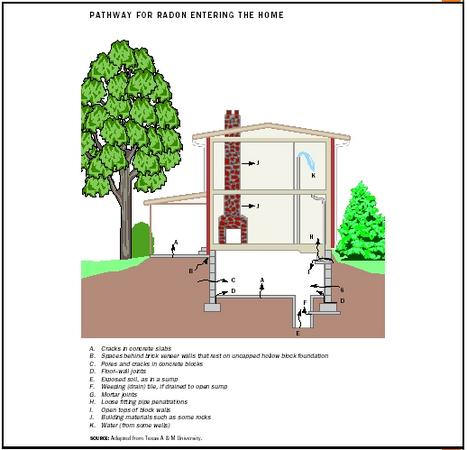
Radon is an odorless, colorless, radioactive, though chemically unreactive
gas. It has an atomic number of eighty-six, which corresponds to the number of
protons found in the nucleus of any isotope of radon. There are more than
thirty known isotopes of radon, and each one emits some combination
of
alpha,
beta, and
gamma radiation when undergoing
radioactive transformation, commonly referred to as "decay."
Radon gas is ubiquitous in the natural environment. This is because the
precursors to radon, such as the aforementioned radium isotopes, and others such
as radium, thorium, and uranium isotopes, are present in some rock formations.
Radon is also found in the man-made environment because many of the materials,
consumer products, and foodstuffs of everyday life come from the naturally
radioactive environment.
Radon is one of the few examples in nature of a gaseous element that results
from the decay of a solid element and then decays into another solid element.
This increases its potentially harmful effect in humans. For example, radon-222,
the most common isotope of radon, is a product of the alpha decay of radium-226
atoms, found in rocks. Radon-222 atoms subsequently produce polonium-218 in a
similar alpha-decay process, and it is this solid substance that can lodge in
human tissue.
Solid-state radionuclides remain where created by decay processes unless they
are redistributed by dissolving in groundwater or by becoming airborne. Given
the chemically inert nature of radon, there are no known compounds that include
this element. Thus isotopes of radon may diffuse away from their place of origin
and usually end up dissolved in ground water or mixed with air above the soil
and rocks that bear their solid precursors.
People's exposure to radon primarily occurs when radon seeps out of air
spaces above soil or rocks and into surrounding indoor or outdoor air, such as
the basements of houses built over radium-bearing rocks. It is not exposure to
radon gas that actually may lead to harm, but exposure to the decay products of
radon, specifically the ones with short half-lives that emit alpha
radiation. Radon-222 offspring, like polonium-218 and polonium-214, become
attached to dust particles that may be breathed in by people exposed to the gas
and become lodged in the respiratory tract. Decay of the radon progeny while in
the lungs is the means by which the radiation dose is delivered to the lungs.
This dose, which is the energy of alpha particles absorbed by cells that line
the lungs, is what gives rise to the potential for lung cancer associated with
exposure to radon.
Radon has been labeled by the Environmental Protection Agency as the
second-leading cause of lung cancer in humans (after tobacco smoke), based on
mathematical risk estimates derived from many published studies of exposure of
subsurface uranium miners to highly elevated levels of the gas, primarily
radon-222. Many radiation health scientists have challenged such findings
because of the vast difference in exposure levels between homes and buildings on
the one hand, and subsurface mines on the other. However, a variety of action
levels and exposure limits for radon gas exposure have been recommended or set
into law for the protection of the public. The Surgeon General and the EPA
recommend that radon levels of four picocuries or more inside homes be reduced.
The EPA states that radon levels less than four picocuries still pose a risk,
especially for smokers.
Methods to both detect and mitigate indoor radon exposure have been devised
as well. Detection and measurement methods usually make use of a device to
collect radon gas atoms or the offspring particles. The simplest real-time
method would be a "grab sample," in which air is drawn into an evacuated flask
that is then taken back to a laboratory for analysis. The most popular
short-term measurement device is the activated charcoal canister, a small
container of steam-treated charcoal that is opened and left at the sampling
location for a prescribed time. Radon is adsorbed by the charcoal, and the decay
products of the radon are analyzed after the canister has been resealed and
retrieved. The simplest mitigation methods include sealing cracks and
penetrations through foundations, as well as diverting the radon away from the
slab or out of the ground, with vacuum or ventilation systems.
National Research Council. (1999). Health Effects of Exposure to Radon—BEIR
VI. Washington, D.C.: National Academy Press.
National Research Council. (1999). Risk Assessment of Radon in Drinking
Water. Washington, D.C.: National Academy Press.
(PRIMAPRESS) ROMA - Giampaolo Giuliani, l'uomo
denunciato per procurato allarme perchè aveva predetto un terremoto
nell'aquilano di grosse proporzioni sbagliando solo di qualche giorno non è
l'unico al mondo a sostenere che attraverso le misurazioni del gas Radon si
possa capire se si sta per verificare un evento sismico di grosse proporzioni.
Da Taiwan agli Stati Uniti e persino dagli esperti giapponesi tale sistema di
predizione dei terremoti da anni è consuetudine. Da numerosi studi compiuti in
zone soggette a rischio sismico è emerso che anomalie nella concentrazione di
Radon nel sottosuolo o nelle acque provenienti da circolazione profonda (o
comunque da sorgenti) sono correlate a variazioni della tensione della crosta
terrestre, e quindi ad eventi di natura sismica. Negli ultimi anni la ricerca
sulla predizione dei terremoti è basata principalmente sull'osservazione di
fenomeni precursori. In ogni caso la correlazione tra terremoti e fenomeni
precursori è ancora di difficile comprensione perché le cause e le condizioni
che li governano sono complesse. Un fenomeno precursore avviene prima che abbia
luogo un terremoto. Negli ultimi venti anni sono stati individuati diversi
precursori, tra i quali la variazione anomala di Radon nel suolo o in sorgenti
situate presso le faglie attive. Il problema più importante che si presenta nel
momento in cui si decide di eseguire una campagna di monitoraggio del Radon è
quello di distinguere il segnale anomalo dall'emissione caratteristica del luogo
o addirittura dal rumore. A questo punto non si capisce bene se l'allarme,
lanciato da Giuliani da diversi giorni, seppur indirizzato alla città di
Sulmona, potesse essere preso meno sottogamba. Sta di fatto che oggi si assiste
ad un tentativo di minimizzare il precedente e di prevenire le polemiche,
dicendo che nessun terremoto si può prevenire.
Eppure basta cliccare sulla frase "Radon earthquake precursor" da
qualsiasimotore di ricerca per rendersi conto che è una pratica diffusa in tutto
il Globo e studiata e pErsino dalle nostre Università. Insomma non basta dire
che non si poteva prevedere e punto. Lo dimostrassero Boschi, Barberi e gli
altri che Giuliani ha colto nel segno per una coincidenza. Fortuna? Coincidenza?
Oppure ben altro. I morti di oggi, se non subito, ma nelle prossime settimane,
obbligano alla massima chiarezza su questa vicenda. E di sicuro Bertolaso non si
sottrarrà ad una simile e necessaria verifica. (PRIMAPRESS)
E ora in Turchia... anche loro lo sanno...
Geochemical monitoring in the Marmara region
(NW Turkey): A search for precursors of seismic activity
Physical and chemical properties of warm and hot spring
waters as well as soil radon concentrations were measured continuously during a
3-year period in the Marmara region; following the devastating İzmit earthquake
of 17 August 1999 (Mw = 7.4). Promising and encouraging anomalies in ground
radon emanation have been recorded and found to be closely related to seismic
activity. The temporal and spatial variations in the soil radon data are
presented. The earthquakes with magnitude >4 in the region were correlated with
positive radon anomalies. Furthermore, during quiescence (absence of seismic
activity) the radon data indicate random walk behavior of radon in soil and show
Rayleigh-type probability density function (pdf), however, during the earthquake
build-up period, the data show deviations from Rayleigh-type pdf. The radon
positive anomalies indicate disturbance of the path of gas movement or gas
release pattern prior to earthquakes. However, systematic and consistent
anomalies in physical and/or chemical properties of the spring waters have not
been detected for earthquakes occurring in the observation period (M < 5.3).
Radon variation in Spring water before and
after Chamoli earthquake,
Garhwal Himalaya, India
V.M.Choubey1, P.K.Mukherjee1 and R.C.Ramola2
1Wadia Institute of Himalayan Geology,
33-General Mahadeo Singh Road, Dehra Dun 248 001, India
E-mail: vchoubey1@rediffmail.com
2Deptt. of Physics, H.N.B. Garhwal University
Badshahi Thaul Campus, Tehri Garhwal -249 001, India
Abstract: Radon levels measured in the springs of Garhwal Himalaya before
Chamoli earthquake (Mb=6.3) of 29th March 1999 have been compared with those
measured immediately after the earthquake. Radon levels in springs are found to
be affected by the earthquake. In all, 39 springs were surveyed for radon which
are divided into three sections across the tectonic structures. The water
discharge data were also collected along with the radon measurements. The
enhancement/reduction of radon concentration and water discharge rate due to the
earthquake were then calculated as Enhancement Factor (EF) by dividing the
pre-earthquake data with that of post earthquake measurements.
It was observed that in most of the springs, radon levels were increased after
earthquake, particularly in worst effected area around Rudraprayag and Chamoli.
Most of the springs that shows very high radon enhancement factor are located in
the vicinity of the different thrusts or maximum damaged zones with development
of ground cracks. Probably, this may indicate that there is some degree of
reactivation of the thrusts and faults present in this area. However, radon
concentrations were found to decrease in some springs. A similar variation was
also recorded for water discharge from the spring before and after earthquake.
The enhancement or depletion of radon and water discharge may be attributed to
the combined effect of earthquake and partial mobilization of major structural
features and lithological control. The effects of earthquake on the radon levels
and water discharge in the springs of Garhwal Himalaya are discussed in details.
A significant change in radon concentration and water discharge from springs in
relation to earthquake shows that this technique may be exploited as an
additional tool in earthquake prediction programme in Himalayan region.
1. Introduction
Himalaya on the whole is experiencing vertical uplift and transverse block
movements due to the compression caused by the continued northward movement of
Indian plate, even after the collision with Eurasian plate in Paleocene. As a
result Himalayan region is being subjected to intense neotectonic movements and
seismic activities. During the past decade two major earthquakes struck in the
Garhwal region alone, i.e., Uttarkashi earthquake [1] of 20th Oct. 1991 (6.5 Mb)
and Chamoli earthquake of 29th March 1999 (Mb 6.3).
Geological and geohydrological signals preceding significant earthquakes have
been reported since 1960 and have been successfully used to predict the 1975
Haicheng earthquake in China. Perceptible changes in terms of hydrogeochemical
parameters have been reported as a result of noticeable earthquake by several
researchers [2,3,4]. During the last few decade, research on seismic precursors
have received enormous attention because of its social relevance. Monitoring of
radon concentration has been found to have a great potential as a reliable
precursor [5]. Several studies suggests that the emanation pattern of radon
(222Rn) can be used as a seismic precursor [6,7,8,9,10,11,12,13]. The emanation
of radon increases with the increasing stress in the crustal layers, and
supposed to be maximum with the release of the stored energy in the form of the
earthquakes. Okabe [14] suggested that along the active faults the soil gas is
enriched in radon. The concentration of radon in air, groundwater, springs close
to the epicentral area increases anomalously just before an earthquake [15].
Deep seated faults and fractures provide passages for migration of the gas and
thereby concentration of radon dissolved in water increases. King [7] observed
high radon near active faults and temporal variations related to large seismic
activity.
The authors have been engaged in radon studies in soil and spring water for last
few years in Garhwal
1
region. The data related to radon concentration in spring water were collected
from this area in May 1997. This forms the basis for the present study to
compare the variation in radon concentration before and immediately after the
recent Chamoli earthquake. However, a more meaningful information can be
extracted if the radon monitoring along with metrological parameters are made on
a continuous basis.
2. Chamoli Earthquake
A moderate earthquake (Mb 6.3) occurred on the early morning hours of March 29,
1999 (0:35:13:59 IST) near the Chamoli town in the higher reaches of Garhwal
Himalaya. Apart from the loss of lives and properties, several ground cracks
have been observed in the vicinity of the area extending up to 1 km in length
with width varying from 10 to 20 cm. Numerous rock falls, landslides and changes
in ground water levels have also been observed after the Chamoli earthquake.
This earthquake was followed by several aftershocks with magnitude up to 5.3.
According to a US Geological Survey report pure thrust faulting has been said to
be the cause of the earthquake based on the focal mechanism solution. It is
worthwhile to mention that the area is traversed by several thrust/faults.
Preliminary reports by the scientists of wadia Institute of Himalayan Geology
suggest that the activation of Main Central Thrust (MCT) seems to be the
causative factor for this tragic event. It may be noted that the Uttarkashi
earthquake of 1991 (Mb 6.5) was also caused by re-activation of MCT.
3. Radon Measurement Technique
750 ml of water sample was taken in radon-tight reagent bottle of 1 litre
capacity connected in a close circuit with a ZnS coated detection chamber
through a hand operated rubber pump and a glass bulb containing CaCl2 to absorb
the moisture. Air was then circulated in close circuit for a period of ten
minutes till the radon formes a uniform mixture with the air and the resulting
alpha activity was recorded. The details of the measurement technique are
discussed elsewhere [16,17]. The calibration factor 1 count/min. = 0.11 Bq/l was
used to convert the recorded alpha counts in Bq/l [18].
4. Regional geology and structure
The geological structure and tectonics of the area has been studied and
published by several researchers [19,20,21,22,23,24,25], however a brief account
of the salient features are presented here.
There are four principal lithotectonic units present in the area affected by the
said earthquake. From south to north ther are: a) Deoban-Barinag formation b)
Rautagara formation c) Ramgarh formation and d) Munsiari formation (Fig.1). The
crystalline rocks of Ramgarh formation forms a large antiformal structure
overlying the Lesser Himalayan rocks. Deoban and Berinag formations to the north
of Chamoli are highly folded into a antiform referred to as Chamoli Window and
inturn is thrusted over by the rocks of the Munsiari formation. The contact
between the two is tectonic, called Munsiari Thrust [20] or MCT-1 [26,23].
Figure 1 Geological map of Chamoli area [after 20] showing radon sample
locations.
5.
In any comparative earthquake related studies on the variation of radon
concentration, it is important to consider the effects due to seasonal and
meteorological parameters. In the present case, however, the data collection
period is almost the same (i.e. May 1997 and April 1999 ). As such, the effects
due to the above factors may be considered as minimum. In order to have a
meaningful comparison, the post earthquake data were collected from the same
springs, as many of them as possible, at the same spot using the same
instrumentation and methodology. In addition, few more springs were also sampled
in the vicinity of the maximum damage zone. In all, 39 springs were surveyed
which are divided into three sections across the tectonic structures. (Table 1
and Fig.1). The water discharge data were also collected along with the radon
measurements (Table 1). The enhancement/reduction of radon concentration and
water discharge rate due to the earthquake were then calculated as Enhancement
Factor (EF) by dividing the pre-earthquake data with that of post earthquake
measurements.
Along Karanprayag–Chamoli-Pakhi section a total of 11 springs were sampled out
of which only 7 were repeated in the post earthquake measurements.
Pre-earthquake radon concentration varies from 0.9 to 35.9 Bq/l as against 1.2
to 68.4 Bq/l observed in post-earthquake measurements with enhancement factors
as high as 26.4 to the lowest of 0.6. It was observed that most of the radon
concentration in spring water and its discharge in this section has invariably
shown some degree of enhancement (EF>1) or remain nearly same, except for the
sample no. eq22. In case of sample no. eq21, however, the discharge rate has
drastically decreased where as the radon enhancement factor is highest (26.4 ).
It may be noted that these two samples lie on the faults of local extent north
of Karanprayag as well as a series of thrusts within a few km radius. The next
highest radon value as well as discharge is also located in the same area
(sample no. eq23).
The post earthquake radon measurements in 8 springs out of total 12 samples were
carried out along Rudraprayag-Tilwara-Okhimath section. The comparison of the
data reveal that the springs located in Tilwara (sample nos.eq3 & eq4) and Kund
(sample nos.eq8 & eq9) show significant enhancement (EF=3.6 to 26.4) of radon as
well as the water discharge (EF=1.2 to 3.0) with the exception of sample no. eq3
where the water discharge has decreased by a factor of 0.25. All these four
samples are again related to the same fault extending from north of Karanprayag
and a couple of thrusts (Fig.1). The Bhatwari–Garponga area witnessed notable
damage and therefore additional measurements were made in the springs of this
section (sample nos. eq11 to eq16). Despite of the increase in water discharge
from springs (samples eq6, eq7 and eq7a), the radon concentrations were found to
decrease. The
reason for the depletion in spite of considerable damage, may be attributed due
to escape of radon gas through the ground cracks that has developed extensively
in this area during the earthquake. The additional water, transported from
non-mineralised area, may also have diluted the radon content in the springs.
In Ghonti-Budhakedar section there are 7 springs that have been sampled in both
the sessions. In addition 5 more springs were also studied during the
post-earthquake measurements. Strikingly the discharge of the spring have
drastically reduced up to 75% (EF= 0.25 to 0.8) after the earthquake. Some of
the previously studied springs have even completely dried up. The earlier
measurements indicate that radon levels were moderately high, ranging between
4.5 to 159.7 Bq/l. In the later measurements, three of the springs recorded
marginal increase in radon contents (EF=1.03 to 3.9), where as rest four springs
have recorded the lower radon concentrations (EF= 0.2 to 0.5). The drying up of
the springs and reduction in discharge rate suggest that there has been a
narrowing down of the fractures and weak planes. This has resulted in the lower
radon concentration due to obstruction of the radon pathways in the subsurface
strata. Probably the emanation of radon might have increased many fold due to
the earthquake in this area, however, it was restricted to a large extent due to
the same reason. It is worthwhile to mention here that uranium concentration in
the granitic rocks near Budhakedar is high [27] and there are reports of uranium
mineralisation also [28]. The anomalous radon concentrations of 622.9 and 106.8
Bq/l, observed in sample nos. eq52 and eq53, respectively, near Budhakedar, are
due to the combine effect of the earthquake and high uranium contents of the
rocks.
Conclusions
The behavior of radon gas built up and its release before and after the
earthquake has been well established based on the continuous monitoring. However,
in the present case, we have collected data a couple of year prior to the
Chamoli earthquake and about a week later. Although we have lost many of the
signatures in between, nevertheless there are some valuable information that can
be drawn based on the available data:
1. There is an overall enhancement of radon concentration in the post-earthquake
measurements of the spring along Karanprayag-Chamoli-Pipalkoti and
Rudraprayag-Ukhimath sections. This is also coupled with an increase in water
discharge rate of springs.
2. The discharge rate of the springs in Budhakedar-Ghonti section have
considerably diminished, even some of the springs studied earlier have dried up.
Except for two springs towards north near Munsiari thrust, the radon
concentration have decreased after the earthquake.
3. Most of the springs that shows very high radon enhancement factor are located
in the vicinity of the different thrusts or maximum damaged zones with
development of ground cracks. Probably, this may indicate that there is some
degree of reactivation of the thrusts and faults present in this area.
The above mentioned results and discussion reveal that there is a significant
relationship between ground water radon concentration and earthquakes. Therefore,
continuous measurements of radon both in soil-gas and spring/groundwater at
several sites in a well organised grid pattern are necessary to make it as
useful precursor in earthquake prediction programme. In addition, the
combination of radon measurements with the measurements of CO2, CH4, N2, H2, He,
Cl and F along with the temperature and electric conductivity of the spring
water may prove a useful hydrogeochemical precursor for any destructive
earthquake.
References
1. Thakur, V.C. and Kumar S. 1994. Seismotectonics of the 20 October 1991
Uttarkashi earthquake in Garhwal, Himalaya, north India. Terra Nova 6, 90-94.
2. Roeloffs, E.A., 1988, Hydrologic precursors to earthquakes–A review: Pure and
Applied Geophysics, v. 126, p. 177-209.
3. Sharma, S.C. 1993. Isotope and geochemical studies on the thermal discharge
in the Alaknanda and Bhagirathi Valleys, Chamoli and Uttarkashi district. Geol.
Surv. Indi. Recd., 126, pt. 8, 211-213.
4. Sharma, S.C. 1997. Thermal springs as gas monitoring sites for earthquake
prediction. In: Rare gas Geochemistry (Ed. H.S. Virk), GND Univ., Amritsar, pp.
193-199.
5. Braitenberg, C., Garavaglia, M., Magnoni, S. and Zadro, M. 1997. Radon and
crustal deformation monitoring in seismic area of Friuli, north-east of Italy.
In: Rare gas Geochemistry (Ed. H.S.Virk), GND University, Amritsar, pp. 143-157.
6. Fleischer, R.L. and Mogro-Campero 1979. Radon enhancement in the earth,
evidence for the intermittant upflow. Geophys. Res. Lett. 6, 361-364.
7. King, C.Y. 1978. Radon emanation on San Andreas Fault. Nature 271, 516-519.
8. King, Y.C., Koizumi, N. and Kitagawa, Y. 1995. Hydrogeochemical anomalies and
the 1995 Kobe earthquake. Science, 269, 33-34.
9. H. Friedmann, F. Hernegger: A Method for Continuous Measurement of Radon in
Water of Springs for Earthquake Prediction. Geophys. Research Letters 5, No.7,
p.565-568, 1978.
10. Wakita, H., Nakamura, Y., Notsu, K., Noguchi, M. & Asada, T. 1980. Radon
anomaly: A possible precursor of the 1978 Izu-Oshima-Kinkai earthquake. Science,
207, 4433: 882-883.
11. Ramola, R.C., Singh, M., Sandhu, A.S., Singh, S. and Virk, H.S. 1990. The
use of radon as an earthquake precursor. Nucl. Geophys. 4, 275-287.
12. Virk, H.S. 1993. Radon and earthquake prediction in India : Present Status.
Nucl. Tracks Radiat. Meas. 22(1-4), 483-494.
13. Virk, H.S. 1995. Radon monitoring of microseismicity in the Kangra and
Chamba Valleys of Himachal Pradesh, India. Nucl. Geophys. 9(2), 141-146.
14. Okabe, S. 1956. Time variation of atmospheric radon content near the ground
surface with relation to some geophysical phenomena. Memoir Sci. Coll. Univ.
Kyoto Sev. A28, 99-115.
15. Duarah, R., Baruah, S., Yadav, D. and Sitaram, M.V.D. 1997. Anomalies in
radon emanation as earthquake precursor phenomena. In: . In: Rare gas
Geochemistry (Ed. H.S.Virk), GND University, Amritsar, pp.175-187.
16. Ramola, R.C., Rawat, R.B.S., Kandari, M.S. and Choubey, V.M. 1997.
Measurement of Radon in drinking water and indoor air. Radiation Protection
Dosimetry, 74(1/2), 103-105.
17. Choubey, V.M. 1998. Radon measurements in soil and water and its relation
with geology, Garhwal Himalaya. In Proceeding volume of the 7th Tohwa
International Symposium “Radon and thoron in the human environment” Japan, (Eds.
A.Katase and M. Shimo) World Scientific Publisher, pp. 193-198.
18. Singh, M., Singh, N.P., Singh, S and Virk, H.S. 1986. Calibration of radon
detectors. Nucl. Tracks-Radiat. Meas., 12, 739-742.
19. Gansser, A. 1964. Geology of the Himalaya. Inter Science Publication. John
Wiley & Sons, 289p.
20. Valdiya, K.S. 1980.Geology of Kumaun Lesser Himalaya. WIHG Publ. Dehra Dun.291p.
21. Saklani, P.S. and Bahuguna, V.K. 1986. Thrust tectonics of the Garhwal
Himalaya. In: Himalayan thrust and associated rocks (Ed. Saklani. P.S.), Today &
Tommorow Pub. New Delhi, 1-25.
22. Roy, A.B. and Valdiya, K.S. 1988. Tectonometamorphic evolution of the Great
Himalayan Thrusts sheets in Garhwal region, Kumaun Himalaya. Jour. Geol. Soc.
India. 32, 106-124.
23. Bist, K.S. and Sinha, A.K. 1990. Imbrication of Main Central Thrust and its
significance in the central sector of the Himalaya. In: Crustal evolution and
orogeny, Ed. S.P.H.
Sychanthavong., Oxford & IBH Publ. Delhi. 293-302.
24. Thakur, V.C. 1992. Geology of Western Himalaya. Physics and Chemistry of the
earth. Pergamon press, 19, (I-VI), 1-363.
25. Metcalfe, R.P. 1993. Pressure, temprature and time constraints on
metamorphism across the Main Central Thrust Zone and High Himalayan slab in the
Garhwal Himalaya. Himalayan Tectonics. Geol. Soc. Special Publication , 74,
485-509.
26. Fuchs, G. and Sinha, A.K. 1978. The tectonics of the Garhwal Kumaun Lesser
Himalaya. Jaharb. Geol. B-A ,121, 219-241.
27. Choubey, V.M., Bist K.S., Saini N.K. and Ramola, R.C. 1999. Relation between
soil-gas radon variation and the different lithotectonic units of Garhwal
Himalaya, India. Applied Radiation and Isotopes. 51 (5), 587-592.
28. Nashine, S.K., Dhanaraju, R., Bhatnagar, G.S. and Narayan Das, G.R. 1982.
Uranium occurrences close to Main Central Thrust around Sileth, Dhargaon,
Chamyala Balganga Valley, Tehri Garhwal (U.P.). Him. Geol. 12., 305-316.
Table 1. Insitu measurements of the Radon concentrations and Water discharge
data during post (April, 1999) and pre(May, 1997)
Chamoli earthquake of Garhwal Himalaya (March 29, 1999)
Radon
Water Discharge
Post-EQ
Bq/l
Pre-EQ
Bq/l
Pre-EQ
Lt/min.
Post-EQ
Lt/min.
Rn-EF
Dis-EF
1. Karanprayag-Chamoli-Pakhi
eq21 68.4 2.6 6 2.5 26.38 0.42
eq22 1.9 3.2 1 0.25 0.59 0.25
eq23 4.5 0.9 2.5 6.0 5.17 2.40
eq24 8.0
eq25 4.2
eq26 27.8 24.3 12 20.0 1.15 1.67
eq28 59.4 35.9 3 5.0 1.66 1.67
eq29 11.3 4.2 5 6.5 2.71 1.30
eq30 1.2
eq31 2.1
eq32 3.0 2.3 6 8.0 1.28 1.33
2.a) Rudraprayag-Tilwara-Okhimath
eq1 0.6
eq3 15.0 3.5 2 0.5 4.27 0.25
eq4 22.8 0.9 15 40 26.44 2.67
eq5 2.1
eq6 56.9 60.0 3 4 0.95 1.33
eq7 6.1 10.2 1.5 3 0.61 2.00
eq7a 5.0 39.7 6 10 0.13 1.67
eq8 219.2 60.4 3 9 3.63 3.00
6
eq9 28.2 7.8 3 3.5 3.63 1.17
eq10 3.4
eq17 25.5 25.8 16 20 0.99 1.25
eq18 4.5
2.b) Subsection: Bhatwari-Garponga
eq11 19.6
eq12 14.6
eq13 97.8
eq14 3.9
eq15 162.4
eq16 61.6
3. Ghonti-Ghansali-Budhakedar
eq41 2.2 4.5 3 2.5 0.50 0.83
eq42 18.5 18.0 4.5 3 1.03 0.67
eq45 5.4 19.5 4.5 1.5 0.27 0.33
eq47 1.9 6.5 0.5 0.29
eq48 1.3 1
eq49 31.9 87.3 3 0.37
eq50 22.6
eq51 10.3
eq52 622.9 159.7 10 2.5 3.90 0.25
eq53 106.8 66.7 6 2 1.60 0.33
EQ=Earthquake, EF=Enhancement factor, Dis.=Spring discharge, Rn=Radon
Misurazioni sull'acqua. Ottimo.
Earthquake Precursors 129 * E-mail: chaddha@ngri.res.in
Precursors for certain earthquakes indicate that, there is
reason enough to believe that precursors do exist and
can be observed for forecasting earthquakes. The concept that catastrophic
damage is the culmination of smaller
events provides a physical basis for the presence of precursors. In case of an
earthquake rupture, certain
precursory activity can be expected, if the observations are made in the near
vicinity of the causative rupture. Even
if they are genuine, the precursors will remain circumstantial, unless linked to
earthquake rupture through a sound theory.
And for this to happen, a study of precursors in seismically active regions is
needed. Application of chaotic dynamics
approach to certain seismically active regions offers some optimism.
Globally, efforts to predict earthquakes were started about a century ago and
peaked during 1970s, when there
was a cautious optimism that reliable earthquake prediction might be possible.
This optimism was mainly due to a few
successful attempts, like the one for August 3, 1973, Blue Mountain Lake
earthquake of M 2.6 in New York based on
the precursory change in the Vp/Vs ratio. The observations appeared to be
consistent with the Dilatancy Hypothesis,
which explains the behaviour of crustal rocks under nearcritical stress levels.
This attempt was followed by another
spectacular and accurate prediction of the February 4, 1975 Haicheng earthquake
of M 7.3 in China based on several
precursors including immediate changes in foreshock escalation and, clustering
and abnormal animal behaviour
in the region. This timely prediction saved about 1,00,000 human lives. But, the
occurrence of M 7.6 earthquake in
Tangshan, China, 14 months later, for which no prediction could be made,
attested to the complexity of earth processes
prior to the occurrence of large earthquakes. Later, when the predicted
earthquake did not occur within the specified
time frame (1985-1993) in the Parkfield prediction experiment in the United
States on San Andreas Fault, the collective
optimism of the scientific community turned into collective pessimism. This
pessimism was further compounded when
a similar effort in Japan, where a prediction had been made for the Tokai region
did not yield positive results. An
earthquake did occur in 2003 in the Tokai region but no definite precursors were
reported prior to this event. Since
then, there are some success stories of definite precursory changes prior to
several moderate to large earthquakes.
These are region specific, for example, shear-wave splitting and in-situ strain
studies in Iceland. Russian seismologists
have been working for several years on statistical and other related approaches,
but have not succeeded in short-term
forecasts.
With the increase in the reporting of precursors, the International Association
of Seismology and Physics of the
Earth’s Interior (IASPEI) appointed a sub-commission on Earthquake Precursors
R.K. CHADDHA*
National Geophysical Research Institute, Uppal Road, Hyderabad - 500 007
Earthquake Precursors for their validation. The subcommission defined a
precursor as a quantitatively
measurable change in an environmental parameter that occurs before main shock
and is thought to be linked to
the preparation of the main shock. Enhanced foreshocks, seismicity pattern,
hydrological and radon gas have been
considered as few of the notable precursors in the recent times. Subsequently,
there has been a debate amongst
seismologists on earthquake prediction. During the 22nd General Assembly of the
International Union of Geodesy
and Geophysics in 1999 at Birmingham, UK, the IASPEI sponsored a symposium on
“Nature of Seismic Sources and
Prediction of Earthquakes”. The proceedings, giving the status of earthquake
prediction related research were
published in 2001 in Tectonophysics. In a joint UNESCOEOLSS publication on
“Encyclopedia of Life Support System”
in 2003, the history on earthquake prediction and provided a glimpse on the
present status of earthquake prediction
(Gupta, 2003). Earlier, in a Special Issue of Current Science in 1992 on
“Seismology in India – An overview” the status
of earthquake prediction in India was discussed in one of the papers. All these
attempts point towards a strong desire
of the scientific community to document and understand the physical phenomena of
earthquakes.
INDIAN SCENARIO
In India, earthquake precursory studies are being attempted at a few research/academic
institutions. DST has
been continuously supporting research projects related to the precursory studies
based on Radon and Helium
measurements, ULF/VLF radio emissions; GPS-based deformation studies, Borehole
observations such as water
level, temperature and other physical parameters in Koyna region, etc. The
notable have been the geomagnetic field
precursory studies in Himalaya and in Koyna by the Indian Institute of
Geomagnetism, Mumbai. Geo-electrical studies
for precursors were studied in the Shillong region. ULF/ VLF magnetic field
emissions associated with earthquakes
are in progress since February 1998 at the R.B.S. College Agra. The Saha
Institute of Physics, Kolkata has been
regularly monitoring the geochemical constituents He Rn, CH4 etc., at Bakreswar
spring and observed anomalies
related to the 26th December, 2004 Sumatra earthquake. However, two systematic
and notable studies in
earthquake precursors are the Northeast India in Himalaya and Koyna region in
Maharashtra. The first study deals with
a medium-term forecast of an M 8 ±½ based on seismicity pattern, which was
considered a moderate success. The
IASPEI Sub-commission on earthquake prediction also reviewed this study. In the
Koyna region various
geophysical, geochemical and hydrological precursors are being
continuously monitored, as this region is a natural
laboratory with earthquakes continuously occurring for the last 40 years.
130 Glimpses of Geoscience Research in India
NORTH-EAST INDIA
On the basis of a study in 1986, which examined the time series of earthquakes
associated with several of the
moderate earthquakes that occurred in the area between 200 N to 320 N latitude
and 870 E to 1000 E a medium-term
forecast was proposed for a possible future earthquake of magnitude 8 + ½
earthquake in the NE region (210 N to
25 ½0 N and 930 E to 960 E) before 1990. This forecast was based on the concept
that moderate magnitude to great
earthquakes in the north-east India region are found to be preceded, generally
by precursory swarms and quiescence
periods. The medium-term forecast came true with a magnitude 7.3 earthquake
occurring on August 6, 1988. The
epicentral coordinates for this earthquake were 25.1490 N 95.1270 E and were
within the proposed region of forecast.
KOYNA REGION EARTHQUAKE PRECURSORY STUDIES
A multi-parametric study has been initiated by National Geophysical Research
Institute, Hyderabad to monitor
seismological, geophysical, geochemical and hydrogeological precursors in Koyna
region. Seismological
precursors are being monitored by a broadband network.
The geophysical precursory studies like gravity, magnetotellurics, electrical
resistivity etc., are also in progress. The
seismological precursory study in Koyna region has led to the proposal of a
nucleation method. The proposed method
is based on the premise of detecting and observing a nucleation zone of
foreshock cluster, which increases over
a time window of 50 to 100 hours period prior to a M~4 to 5 earthquakes. Studies
on the deepening of such a zone
to foresee a hypocentre of a future moderate-size earthquake at the base of the
seismogenic layer. Three successful
predictions of moderate-size earthquakes in the Koyna region during 2006-07 have
been made by National
Geophysical Research Institute base on the nucleation concept. Precursor studies
for monitoring well water levels
in deep bore wells in the Koyna region have resulted in the identification of
pre and co-seismic precursors for
earthquakes of magnitudes > 4 occurring in this region.
Radon is being continuously monitored at three sites in the vicinity of the
epicentral region in Koyna. The analysis of
data showed a sudden increase in Radon anomaly by a factor of two, about 19 days
prior to 14th March 2005
earthquake (M 5.1) in the region. The Ministry of Earth Sciences, Government of
India has taken a major initiative
to establish Multi-parametric observatories to monitor precursors in certain
seismically areas in the country.
Two such observatories are already in operation at Ghuttu in Himlaya, being
operated by the Wadia Institute
of Himalayan Geology, Dehradun and the other at Koyna, operated by the National
Geophysical Research Institute,
Hyderabad. Similar, observatories are being planned in Andaman and Nicobar
Islands and Northeast India.
REFERENCES
Chadha, R.K., Pandey, Ajeet P. and Kuempel, H.J., 2003, Search
for earthquake precursors in well water levels in alocalized
seismically active area of Reservoir Triggered Earthquakes
in India: Geophys. Res. Lett., v. 30 (7), p. 1416, doi:10.1029/
2002GL016694.
Das, Nitish, K., Bhandari, Rakesh, K., Ghose Debasis, Sen
Prasanta and Sinha Bikash, 2005, Anomalous fluctuation
of radon, gamma dose and helium emanating from a
thermal spring prior to an earthquake: Current Science,
v. 89(8), p. 1399-1404.
Gupta, K.H. and Singh, H.N., 1986, Seismicity of the north-east
India region: Jour. Geol. Soc. India, v. 28, p. 367-406.
Gupta, H.K., 1992, Seismology in India: An overview: Current
Science, v. 62 (1, 2).
Gupta, H.K., Chadha, R.K. and Srinagesh, D., 2001, The Nature
of Sources and Prediction of Earthquakes: Tectonophysics,
v. 338(3,4), p. 357.
Gupta, H.K., 2003, Nature of earthquakes: Publishers Joint
UNESCO-EOLSS, p 58.
Gupta H.K. et al., 2006, An earthquake of M~5 may occur at
Koyna: Curr. Sci., v. 89 (5), p. 747-748.
Gupta, H.K. et al., 2006, Prediction of an M~4 earthquake in
the Koyna region comes true!: Jour. Geol. Soc. India,
v. 68, p. 149-150.
Gupta, H.K. et al., 2007, Earthquake forecast appears feasible
at Koyna India: Curr.Sci., v. 93(6), p. 843-848.
Reddy, D.V., Sukhija, B.S., Nagabhushanam, P. and Devender
Kumar., 2004, A clear case of radon anomaly associated
with a micro-earthquake event in a Stable Continental
Region: Geophy. Res. Letters, v. 31, L10609.
Singh, B., Kushwah, V., Singh, V., Tomar, M. and Hayakawa,
M., 2005, Simultaneous ULF/VLF amplitude anomalies
observed during moderate earthquake in Indian region,
Indian: J. Radio & Space Phys., v. 34, p. 221.
Singh, R.P., Singh, B., Kushwah, V.K. and Chauhan, R.V.S.,
2004a, Attenuation of ULF-VLF seismo- electromagnetic
signals and their propagation to long distances: Indian
J. Radio & Space Phys., v. 33, p. 189.
Singh, B., Kushwah, V., Singh, O.P., Lakshmi, D.R. and Reddy,
B. M., 2004b, Ionospheric perturbations caused by some
major earthquakes in India: Phys. Chem. Earth, v. 29,
p. 537.
Jedi Simon
Ora scusatemi ma c'e un 4,2 in corso e continuo la ricerca appena posso....
vado....
Passata per ora...fiuuuu....
Ora associamo all'analisi dinamica del gas, l'analisi del
campo elettro-magnetico per consentire un controllo incrociato di dati,
comparati
al fine di definire con maggiore certezza e precisione riguardo al luogo e
all'ora nella quale avrà luogo l'evento distruttivo. Con grande ringraziamento
a Dionysios Dimakos (SV1ZJ)
EARTHQUAKE PRECURSORS
By Dionysios Dimakos (SV1ZJ)
I am 38 years old and I reside in
Athens, Greece. My major is electronic engineering. Since 1991, I have been
involved – as an amateur - in monitoring and recording the magnetic field
variations, aiming to trace earthquake precursors. For this purpose, I have
constructed and tested many different circuits and sensors. It is a fact that
the major problem during measurements is created by the use itself of electric
devices, as well as the power lines.
Scope of Measurement
During the past few years, I have focused my study on 0,1
Hz to 40 Hz frequency spectrum, measuring and recording the instant variations
of the magnetic field and not its absolute value.
Unfortunately, in the vicinity of big cities, the levels of
signals from natural sources are 1.000-30.000 times lower than those of signals
transmitted by our technological civilization. For this reason, the use of
filters in the electronic circuit is imperative.
The Electronic Circuit
The electronic circuit diagram can be seen on Picture 1
and Picture 2.
It consists of amplifying stages and electronic frequency
filters.
Its first stage consists of the operational amplifier
LT1128. The alternative voltage (in the 50Hz frequency) of the LT1128 Pin 6
should not exceed +-2V (in reference to ground); alternatively, we reduce the
value of R1.
The second stage is a filter “Notch” in the frequency of
50Hz and consists of two OP27.
The three variable resistors of the filter are 20-turns “trimmers”,
adjusted to the values specified on the diagram, before placed on the circuit.
When the circuit is in operation measuring the magnetic field, the “trimmers”
are readjusted micro metrically on the original values, in order to achieve the
lowest AC voltage in the frequency of 50Hz, at the circuit output.
From “trimmer’ R2, we should have 0 V DC at the circuit
output, while from the “trimmer” of the output stage, we adjust the value of the
output signal which we forward to the Line-In of our computer sound card.
The capacitors C1, C2, C3, C4 are of “Silver mica” or
“foil polystyrene” type in order to maintain stable capacity during temperature
variations.
All stable resistances are of “metal film” 1% type.
Having tested many different operational amplifiers
combinations, I decided on the ones of the diagram since they offer lower noise
levels and better overall performance on the specific circuit.
The Sensor
The sensor consists of a 50cm long ‘PVC’ pipe, with 5cm
external diameter. We wrap three layers of 0.04’’ “MuMetal” sheet around the
pipe. Over the “MuMetal”, we wrap insulating tape and coil enamel coating wire,
1 mm thick, at pipe's length. We coil ~9 layers of wire (~ 4.500 coils). When
the coil is completed, we wrap it up with insulating tape and plate it with
aluminum foil or self-adhesive aluminum tape. The aluminum is connected to the
plate of the coaxial cable (RG-213, RG-8…) that we use as signal transfer line.
 |
|
The end of the external winding of the coil is also
connected to the shield of the cable, while the internal end is connected to the
internal conductor of the coaxial cable. The coil in inserted into a 60cm long
‘PVC” pipe, with 10cm diameter it is then stabilized and waterproofed.
The coil has pure resistance R = 16 Ohm and
self-induction L = 1 H. The final construction is placed horizontally 10cm
above the ground and stabilized. The ends of the coil are adjusted at 110o and
290o respectively in reference to the magnetic north. . |
Just to emphasize that the coil should have low pure
resistance (including the coaxial cable), in order to achieve reduced noise in
the circuit
Recording Software
For the recording, I use the “spectrogram” with the
following settings:
- Line in: to maximum sensitivity
- Screen Resolution : 1152 x 864 x 16 bpp
- Tracing Form F.F.T
- Signal scale: - 30 db
- Sample rate: 5,5 KHz 16bit
- F.F.T. points : 16.384,
- Linear frequency scale
- Average count: 1
- Pitch Detector: off
- Time scale: 6250 msec
In order to save the images, I use program “2020” with the
following settings:
- Capture: Desktop – scrolled area
- Auto save
- Auto increment
- PNG (Image format)
- Time capture: 7200 sec (2 hours)
- Rectangle Repeat
Receiving Samples
28_4_2003
Record
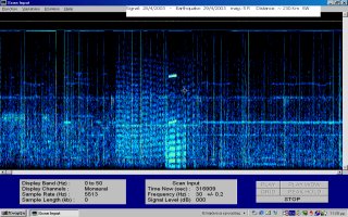
Quake 29_4_2003,
5R 230km SW |
|
8_6_2003
Record
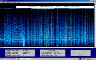
Quake 9_6_2003,
5R 230km NNW |
|
|
|
6_7_2003
Record
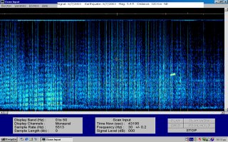
Quake 6_7_2003,
5.4R 320km NE |
|
13_8_2003 Record
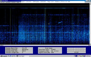
Quake 14_8_2003,
5.9R 275km WNW |
|
|
|
8_2_2004
Record
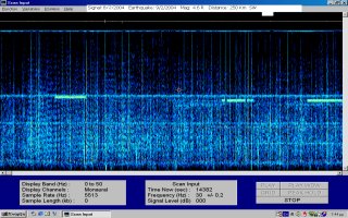
Quake 9_2_2004,
4.6R 250km SW |
|
29_2_2004
Record
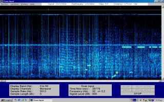
Quake 1_3_2004,
5R 175km SW |
|
|
|
07_3_2004
Record
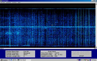
Quake 11_3_2004,
4.5R Dodecanese Isl |
|
14_3_2004
Record
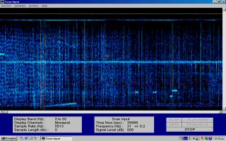
Quake 17_3_2004,
6.1R South of Crete Isl |
Findings
I have already completed an analysis of the records
produced during the period from 01-02-2003 to 01-03-2004. (During that period,
the reception/ recording device has been unavailable for a total of 30 days due
to technical reasons.)
According to Athens National Observatory, 12 earthquakes
of 4,8R or above have been recorded for the same period. (Aftershocks that
follow bigger earthquakes within a few days are excluded; earthquakes that
occurred the days from 23-07-2003 till 26-07-2003 are also not recorded due to
technical problem.)
Analyzing the remaining 10 earthquakes in relation to the
registered precursors, we can draw the following conclusions:
- 60% of the earthquakes occurred within 24 hours from the
initiation of the earthquake precursors
- the remaining 40% of the earthquakes occurred the next
2-7 days
- although a number of precursors have been recorded
during morning or afternoon hours, the majority is recorded between 17:00 and
22:00 local time
- no precursor has been registered between 23:00 and 08:30
local time
- the average time of the precursor reoccurrence is app. 7
days
Studying all precursors that have been recorded the past 14
months as well as the earthquakes that followed, we can draw the following
conclusions:
1. The time of precursor occurrence is somehow related to
the positions of the Sun and the Moon in relation to Earth and the gravitational
powers generated. A signal possibly related to a forthcoming earthquake is twice
as likely to appear within 72 hours after the actual time of each phase of the
Moon (new moon, first quarter, full moon, last quarter), than within the 72
hours before.
2. The average time of occurrence is app. 1 hour before
sunset
3. 75% of the earthquakes
following the precursors occur within 72 hours after the precursors
Earthquake Precursors Pattern
The pattern of earthquake precursors could be described
as “pre-earthquake signature” since every reoccurrence maintains common
characteristics. Observing the recorded signal, one realizes that, throughout
the spectrum 1-40Hz, there are lines almost parallel to each other at any given
time. Any spectral line differs 1-3Hz from the previous one.
The duration of the “pre-earthquake signature” varies
from 15 minutes up to 3 hours, while for the specific spectral impressions, the
intensity of the magnetic field varies from 2 PT to ~20 PT. It is most likely
that the common characteristics of the signal will still appear in frequencies
higher than 40 Hz. Further observation is required in order to verify the
following:
What is the correlation of the magnetic field intensity
and the duration of the “pre-earthquake signature” with the data of the
earthquake to follow?
What is the highest frequency in which the “pre-earthquake
signature” is observed, as well as the correlation of the frequency with the
earthquake magnitude or the distance from the epicenter to the reception device?
Conclusion
The intensity of the earthquake precursor will be
increasing as one approach the epicenter of the imminent earthquake.
Consequently, earthquake prediction through the method described above requires
a network of base-stations throughout the country, each station including at
least two sensor devices and the respective recording equipment.
I believe that observation of the earthquake “signature”
used in parallel with other methods can provide very satisfactory results in
earthquake prediction.
Teamwork, selfless interest and publication of the progress
and research findings of different scientific groups are the prerequisites for
successful earthquake prediction. Selfish motives can only cause further delay
to a possible solution, which means more death and tragedy….
I hope that soon all scientists working in the specific
field will cooperate and combine their knowledge in order to achieve a common
goal, earthquake prediction, which is essential to humanity.
In the future, “pre-earthquake signatures” will be posted in
this site, as soon as possible following occurrence.
We are always at your disposal to provide further
clarifications and data to anyone interested in constructing the specific device.
More detailed pictures are available at my web site:
http://www.ham.gr/ulf/index_en.php
Qui puoi trovare gli spettrogrammi degli ultimi terremoti.
EARTHQUAKE TRIGGERING, EARTHQUAKE PRECURSOR SIGNAL
GENERATION,
AND EARTHQUAKE SENSITIVITY THEORY PICTURES
Latest Update: May 20, 2004
Earthquake
Triggering
Earthquake
Precursor Signal Generation
Earthquake
Sensitive Humans, Animals, And Plants
Earthquake Triggering Forcess Reference
Information
Variabili da tenere presenti
nel calcolo delle previsioni, per l'analisi della somma di tutti i vettori e di
tutti gli elementi che possono prendere parte alla costruzione di un'onda
sismica.
Site visitors are invited to make suggestions regarding additions to
or corrections to these general theory pictures. Please send the suggestions to:
seismic@ix.netcom.com.
Many of the individual theories outlined here have been proposed by and
discussed by researchers around the world over the years.
And one goal is to try to locate and
include references to as many of those researchers’ publications as possible.
EARTHQUAKE TRIGGERING
The following theory pictures propose how earthquakes are
being triggered. Just a few of the most important earthquake triggering forces
and phenomena are being discussed. A number of others are listed in the
following report:
Earthquake Triggering Processes.
A - 1 The movement of tectonic plates
relative to one another and other processes cause strain to build in
earthquake fault zones around the world.
A - 2 Various obstacles such as the
resistance of rock layers to smoothly slip past one another cause that
strain energy to build to dangerously high levels in some fault zones.
A - 3 Enough strain eventually accumulates in the
fault zone rock layers to overcome those obstacles.
And some of that stored energy is released in the
form of a powerful earthquake.
A - 4 Two groups of forces, phenomena, and factors which can
affect earthquake triggering are ones related to the
gravitational pulls of the sun and the moon on the Earth, and fault zone
environmental factors such as it north and south or east and west
orientation.
A - 5 External forces or phenomena such as
atmospheric storm related wind drag on continents
and fault zone rock layer heating associated with solar
and geomagnetic storms can temporarily or permanently
add or subtract sufficient amounts of strain energy
to or from the fault zone to
move an earthquake occurrence time forward or backwards hours, days, or weeks in
time.
A - 6 Forces or phenomena such as
shockwaves from powerful earthquakes occurring around the world or
nuclear tests can produce permanent instabilities
in a fault zone and move the earthquake occurrence time forward or backwards
days, weeks, months, decades, and even centuries in time.
A - 7 The actual earthquake occurrence time window is often
finally determined by strain which is temporarily or permanently added to the
fault zone by forces or phenomena which are directly
and/or indirectly associated with the gravitational pulls of the sun and
the moon. Some of those phenomena would be ocean tides and
the Solid Earth Tide.
The following drawing shows how forces related to the
gravitational pulls of the sun and the moon on the Earth's crust can trigger an
earthquake. A fault zone running east and west (EW) may fracture when the
gravitational pulls of the sun and the moon pull it towards the north and the
south at the same time. And a fault zone running north and south (NS) may
fracture when the gravitational pulls of the sun and the moon pull it towards
the east and the west at the same time.

A - 8 Two specific earthquake triggering force related
theories are presently being considered. The first (see
D – 1)
involves earthquake triggering pressure being directly
exerted on the Earth’s crust by the gravitational pulls of the sun and the moon.
The second (see
D – 2)
involves earthquake triggering pressure being exerted on
the crust by the Earth’s solid core as it attempts to move away from the
sun – Earth – moon barycenter or center of mass which the core, the crust, the
Earth as a whole, and the moon rotate around once each month.
A - 9 When forces or phenomena such as atmospheric and
earthquake related shockwaves move the earthquake occurrence time forward or
backwards in time from when it would have ordinarily occurred then the
occurrence time shifts to another distinct time window which is controlled by
the gravity related forces. Shift like that do not involve arbitrary amounts of
time.
A - 10 Sun and moon gravity related forces and phenomena can
reach high and low strength points in a number of different time cycles. Several
of the most important cycles are multiples of roughly 6.25 hours (including 24
hours and 50 minutes) and multiples of about 7 days (including 28 days).
A - 11 A number of cycles having the same time length can be
active at a given time. For example, one 6 hour cycle may be controlled by the
position of the moon in the sky while at the same time another 6 hour cycle is
controlled by the location of ocean tide crests and troughs.
A - 12 Which time cycles control occurrence times for
earthquakes in a given fault zone system is strongly related to how forces and
phenomena related to the cycles cause different rock layer sections in the fault
zone system to be bent, stretched, or compressed in relation to one another.
Another way of saying that is to state that what might be described as time
cycle controlled Pressure Waves within the Earth's crust are actually
triggering most earthquakes.
A - 13 It has been proposed by at least one researcher that
in most cases earthquake occurrence times are linked with points of high and low
strain in the time cycles while a smaller percentage of earthquake occurrence
times are linked with the times when time cycle related earthquake triggering
forces are experiencing their most rapid change in strength.
A - 14 Earthquake aftershocks are often not random events as
far as their occurrence times are concerned. Those times are frequently
controlled in part by those sun and moon gravity related time cycles. In fact,
the aftershocks are even more likely to be controlled by them than the original
earthquake.
EARTHQUAKE PRECURSOR SIGNAL GENERATION
Only a few earthquake precursor signal generation related
processes are being discussed here.
B - 1 Phenomena such as the
piezoelectric effect cause different types of
electromagnetic energy field fluctuations to be generated in fault zones
in the days, weeks, months, and years before earthquakes occur.
B - 2 Geomagnetic storm energy
(which often has its origins in solar storms) can interact with fault zones and
in the process contribute to or amplify certain fault zone activity related
electromagnetic energy field fluctuations.
B - 3 Solar storm activity is
associated with events taking place in and around the sun. Interactions between
solar storms and the Earth's geomagnetic field and earthquake fault zones are
affected by the nature of the solar storm and also
the orientation of the sun's magnetic field lines relative to those of the Earth.
About every 7 days the sun magnetic field lines orientation can shift from
being in the same direction as those of the Earth to being in the opposite
direction.
B - 4 Earthquake fault zone activity related
electromagnetic energy fields can be focused in
specific directions by a variety of phenomena. As a result before an earthquake
a sensor located a certain distance on one side of the fault zone might be
detecting strong energy field fluctuations while another one an equal distance
away on the fault zone's other side might not detect anything. This is one of
the important reasons that some energy field detectors give the appearance of
not producing consistent results.
B - 5 The geomagnetic storm - earthquake fault zone
interactions take place most often during the days and weeks just before an
earthquake occurs when the fault zone’s rock layer's physical, chemical, and
electrical properties change as it gets close to fracturing. But they can also
take place months and perhaps years before the earthquake occurs.
B - 6 Phenomena such as lighting strikes and I believe
geomagnetic storms can cause low frequency radio waves to be generated. I expect
that events taking place within fault zones can also cause them to be generated.
Those radio waves can travel around the world with
relatively little loss in signal strength. Air is a reasonably good conductor
for them. Water is better. And metal is best.
As they interact with fault zones and/or when they are
generated as the result of fault zone activities, information regarding fault
zone events can be superimposed on them and then be carried by them around the
world.
B - 7 Some fault zone event related electromagnetic energy
field fluctuations range in time from 0.25 seconds to perhaps 30 seconds in
duration. Others may persist for hours, days, and even weeks.
B - 8 Because the times when those energy field fluctuations
occur can be controlled by forces or phenomena related to the gravitational
pulls of the sun and the moon and also forces or phenomena related to
geomagnetic storms etc., the fluctuations can occur at high strain level times
etc. in the same time cycles which control earthquake occurrence times. Or they
can occur at somewhat random looking times which may be days, weeks, or months
apart.
B - 9 Other earthquake precursors possibly related to
electromagnetic energy field fluctuations have been reported over the years.
They would include Earthquake Lights which
are a type of temporary, local luminescence, glowing
balls of light which may be suspended in the air,
and static noise on radio, television, and
telephone transmissions.
B - 10 Interactions taking place between earthquake fault
zones located even great distances apart can result in
signals being generated which are stronger than they might otherwise be.
For a hypothetical example, an approaching 8.0 magnitude earthquake in one fault
zone might cause a signal associated with a 4.0 magnitude earthquake which is
about to occur in another, distant fault zone to be amplified to a point where
it appears to be for a 6.0 magnitude earthquake.
EARTHQUAKE SENSITIVE HUMANS, ANIMALS, AND PLANTS
C - 1 Electromagnetic energy field fluctuations linked with
fault zone events and in some cases also with low frequency radio waves which
are affected by or generated as a result of fault zone events, can produce
strong reactions in humans, animals, and perhaps some plants.
C - 2 Various groups of organisms such as dogs and catfish
will have different types of and different levels of sensitivity to those energy
field fluctuations. And within a single group of organisms such as dogs
different members will experience different types of and different levels of
sensitivity to those energy field fluctuations.
C - 3 The responses of different organisms to the energy
field fluctuations can result from basic energy field - biological system
interactions. Those types of interactions would be similar to having water
heated by the energy field of a microwave oven.
C - 4 They can result as side effects of energy field -
biological system interactions which the evolutionary process has deliberately
built into the members of a specific group of organisms for some reason such as
to provide them with an ability to detect light or to sense the orientation of
the Earth's magnetic field.
C - 5 They can result from energy field - biological system
interactions which result from a deliberate effort by the evolutionary process
to provide the members of a specific group of organisms with an ability to
detect the approach of an earthquake.
C - 6 I have never heard about any research being done on
plant sensitivity to those energy field fluctuations and am simply assuming that
such effects probably exist.
C - 7 Earthquake sensitive animals may become temporarily
agitated and/or disoriented by those energy field fluctuations. Some pet animals
may wander away from home and become lost.
C - 8 Animals respond mostly to energy field fluctuations
which are linked with events taking place in local earthquake fault zones.
However, an occasional animal will be able to sense those fluctuations when they
are associated with fault zones which are hundreds of miles away.
C - 9 Some pet animals which might behave as though they are
earthquake sensitive are actually responding to fault zone activity related
behavioral changes etc. which they are observing in their earthquake sensitive
human owners.
C - 10 All humans are probably earthquake sensitive to some
degree. Some fraction of the population is sufficiently sensitive to be able to
clearly tell when a local earthquake is going to occur. A small fraction are
sufficiently sensitive to be able to detect signals associated with earthquakes
occurring around the world.
C - 11 Earthquake sensitive humans may experience physical,
random or monthly type hormonal, emotional, and brain activity related responses
to those energy field fluctuations. Headaches are among the most common
responses. Nausea and dizziness can occur. Some people may experience abrupt,
strong, and temporary or even somewhat longer lasting mood swings. High or low
frequency tones may be heard in one ear or the other or in both ears at the same
time. Short duration muscle jolts are common. Physical pain or some other type
of sensation in a hand or foot and in extreme cases actual physical injury can
occur. Dreams may be influenced by those energy field fluctuations. Especially
sensitive people may begin hearing voices or seeing ghostly images. I believe
that some people might begin seeing auras of different colors surrounding other
people.
C - 12 Some earthquake sensitives can determine from which
hand or foot is being affected by those energy field fluctuations etc. roughly
where on the planet an approaching earthquake is likely to occur.
C - 13 Because water is a good conductor for the low
frequency radio waves, earthquake sensitive humans will sometimes experience
stronger reactions to the fault zone activity related energy field fluctuations
when they stand near a large body of water such as on the ocean shore. Their
reactions may get abruptly stronger when they stand near metal water pipes in a
house and even when they begin running tap water into the kitchen sink.
C - 14 People who have water dowsing abilities are probably
often detecting those energy field fluctuations as the signals travel through
underground sources of water. I understand that dowsers are not usually able to
detect the presence of electrically isolated bodies of water such as water
present in a plastic swimming pool.
C - 15 Diet modification and dietary supplements can at
times be used to control painful headaches or other undesired responses to those
fault zone activity related electromagnetic energy field fluctuations. Common
pain control medications such as aspirin may help. People who are strongly
earthquake sensitive may need to rely on prescription drugs. Certain types of
medications and foods can temporarily increase a person's sensitivity to the
energy field fluctuations.
Biofeedback can reportedly help reduce earthquake
sensitivity. And I would expect that hypnosis might also work for some people.
Some earthquake sensitives have reportedly been able to
reduce the number and severity of their headaches or mood shifts etc. by moving
to some other part of the country where fault zone activity related
electromagnetic energy field fluctuations are weaker or at least different.
After such a move it might require several weeks for the undesired energy field
related responses to be reduced in strength.
C - 16 An inexpensive and effective way to detect
approaching earthquakes might involve having a number of people who are
earthquake sensitive contact some central facility when they were having
earthquake warning experiences such as headaches. If 100 in some area were
reporting in and only few in surrounding areas were doing the same then that
might be a sign that an earthquake was about to occur near that first area.
Additionally, earthquake forecasters and researchers could always ask them for
more information when desired. That is obviously not possible with earthquake
sensitive animals or conventional radio signal receivers or seismic activity
monitors. See: A
Demonstration Earthquake Prediction Program
EARTHQUAKE TRIGGERING FORCES
D - 1 An External Source Of
Earthquake Triggering Pressure On The Earth’s Crust
As the following drawing shows, the Gravity Point
is the location on the surface of the Earth where the combined gravitational
pulls of the sun and the moon are strongest.

As the Earth rotates each day on its North and South
Pole axis, its crust on the side which is rotating towards the Gravity Point
is accelerated by the sun and moon gravity while the side moving away from the
Gravity Point is decelerated or slowed. That creates strain within the
crust. And earthquakes are triggered at locations where that strain causes the
crust to be bent, stretched, or compressed in just the right directions.
D - 2 An Internal Source Of
Earthquake Triggering Pressure On The Earth’s Crust
As that previous drawing shows, once each month the
Earth and the moon rotate around a sun – Earth – moon barycenter or center of
mass which is a certain distance down beneath the surface of the Earth. The
location of that barycenter is constantly moving towards and away from the
center of the Earth depending upon the location of the sun relative to the moon.
And it is constantly moving around the location of a line drawn between the
center of the Earth and the center of the moon.
The solidified iron believed to be the major component
of the Earth’s core is roughly 5 times as heavy or dense as the material in the
Earth’s crust. As both the core and the crust rotate around that barycenter once
each month the mass of the Earth in general attempts to assume the shape of an
egg with its ends pointing away from the barycenter. And the solid core tries to
move in a direction almost directly away from both that barycenter and from the
location of the moon.
The Earth’s gravity, rotation, and its somewhat rigid
structure prevent it from undergoing rapid, appreciable changes in shape. And
the core is kept from moving within the Earth by those factors. That results in
the solid core exerting earthquake triggering pressure at different locations or
pressure points in the crust from inside the Earth. Where those pressure points
are located is determined by factors such as the location of center of mass of
the core relative to the sun – Earth – moon rotation barycenter and the
rotational orientation of the Earth as it revolves once each day on its North
and South Pole axis.
REFERENCE INFORMATION
How Earthquake Sensitives Predict Earthquakes, GeoMonitor: Earthquake
Prediction News; April, 1996
Breathing of the seafloor: Tidal correlations of seismicity at Axial
volcano, Geology; June 2002; v. 30; no. 6; p. 503-506 (See especially Figure
4A.) (Also, that paper contains a helpful list of references.)
'Restless Earth' May Give Advance Notice Of Large Earthquakes (NASA
News)
Prediction of Destructive Earthquake by the MDCB-Method, Wang,
Wen-xiang and Yang, Wu-yang, Xian Sub-Institute, Coal Science Research Institute
of China MDCB Web Site
Cellphone can warn of earthquake
The
7.4 magnitude devastating earthquake in Pakistan on October 8 has raised several
questions and posed new problems for scientists and engineers.
It is for the first time in
seismic history that military personnel inside bunkers have been killed.
There have been cases before of
soldiers killed in earthquake while overground. But the present case is unique
and military engineers will now have to revise their design to make bunkers safe
against seismic forces.
But the most frequently asked
question is whether it is possible to predict the occurrence of an earthquake.
The answer to
this question is, 'yes, to a sufficient degree of accuracy, about a few hours
before the occurrence of an earthquake.'
Complete coverage:
Tremors across borders
The earthquake precursors
discussed here are exclusively for moderate to large earthquakes, meaning
earthquakes of magnitude 6.0 or more on the Richter Scale. Earthquakes of lesser
magnitude may or may not necessarily exhibit all the precursors.
Earthquake precursors have been
divided into three broad categories. a. long term precursors.
This means more than five years in advance; b. medium term
precursors. This means within about four to six months in advance; and
c. short term precursors. This refers to signs within 20 to 30 hours.
Long term seismic
precursors: The location and magnitude of the likely epicentre is
calculated based primarily on statistical studies, and the prediction is
probabilistic. It is reliable when the probability of occurrence in the next
five years or less is more than 0.6. However, such predictions are more useful
to academic professionals and researchers.
Medium term precursors:
Such predictions are able to give the location of the quake to a sufficient
degree of accuracy, and the likely time of occurrence and magnitude are somewhat
grotesque. The period of six months or so could be used for creating seismic
awareness, taking suitable mitigatory measures, imparting seismic training to
various forces etc. These are indicative of changes in the
geomagnetic field, changes in the gravity field, rise in sub-surface
temperature, rise in ground radioactivity etc. All these measurements indicate
that something is wrong inside the earth. But it is not possible to
arrive at any definite inference. Inputs from such parameters are useful to
administrators and academicians.
Short term precursors:
These could be seen by the common man and are highly
reliable. People in seismically active areas may keep a copy of this
article for further use. There are several types of short term precursors which
could be seen and observed by different strata of society.
Thermal precursor: A few months before the occurrence of an earthquake
the average temperature of the area keeps increasing. Weather report
bulletins refer to temperatures above or below average by so many degrees. It is
seen that in case the area is heading for an earthquake, the average temperature
goes on increasing. On the day of the earthquake it is
about 5 to 9 degrees Celsius above the average normal temperature for
that day. This could be monitored by the meteorology
department and also by thermometers inside homes.
Water precursor: There is a sudden rise or fall in water level in the
wells. It could be as high as one metre. Sometimes
the well water may turn muddy. At times a fountain appears inside the
well. All these changes happen about one or three days
before the earthquake. Sometimes a fountain appears
in the ground. This normally happens a few hours before the quake.
The Gujarat earthquake of 2001
Another
form of water precursor is seen in the flow of riverwater.
There is a sudden and rapid increase or decrease of water
flow in the river or nallah. This happens about
one to two days before the quake.
Seismo-electromagnetic precursor: This is a very reliable
precursor. It occurs and is exhibited about 10 to 20 hours
before the quake. Before the occurrence of an earthquake the subsurface
temperature rises. As a result of this the geomagnetic field is reduced. The
reduction in geomagnetic field adversely affects the propagation of
electromagnetic waves. This is experienced abundantly on the radio, television
and telephone.
If one is
tuning the radio at 1000 kHz, then the same station will be received in the
potential epicentral area, about 10 to 30 hours before the quake, at higher
frequencies. Maybe 1100, 1200, 1300, 1800, 1900, 2000 kHz or so.
Similarly, reception on
television is affected by audio, visual and spectral disturbances. The
telephone's reception is also adversely affected and there is a continuous
disturbance that you can hear.
Apart from this, a recent
reliable precursor is the mobile telephone. It has been found that about
100 to 150 minutes before the occurrence of an earthquake,
mobile telephones start non-functioning or malfunctioning. The timespan
indicated is sufficient to take all necessary mitigatory measures.
A word of caution: all the
above precursors are valid only when seen and manifested extensively. Failure of
one or two instruments should not be taken as a seismic precursor.
Animal precursor:
It is seen that 10 to 20 hours before the occurrence of an
earthquake, the entire animal kingdom becomes highly disturbed and restless.
They move in a directionless manner and in fear. Birds
do not sit on trees but move about at a low height,
emitting a shrill noise. Rodents like rats, mongooses etc are in a panic.
Domestic animals like cows, dogs, cats etc struggle against being tied up, and
even turn on the owner.
Human precursor:
Doctors and nurses observe that some sensitive patients in hospitals become
highly disturbed. They exhibit a sudden rise in blood
pressure, heart trouble, headache, migraine, respiratory
disorders etc. Further, these psychosomatic signs
are manifested without any provocation. It is also seen that the number of
patients in the out-patient department increases by five to seven times, some 10
to 20 hours before the quake.
The best
indicator is the number of child deliveries in any hospital. On the penultimate
day of the earthquake the number of deliveries goes up about three to five
times, while on the day of the earthquake it is as high as
seven to eight times the normal.
Arun Bapat is a
research seismologist. He was formerly Head, Earthquake Engineering Research
Division at the Central Water and Power Research Station, Pune. He can be
contacted at:
arun_bapat@vsnl.com
Just prior to an earthquake, the birds go to the bottom of
the cages and huddle in a corner.
Air-borne ions have reportedly a pronounced biological impact on humans
and animals (Charry, 1984; Krueger & Reed, 1976). Exposure to negative ions
is generally perceived by humans as pleasant, may enhance the cognitive
performance, and has overall beneficial health effects (Baron, 1987). By
contrast, positive ions elicit adverse reactions including headaches, nausea,
depression, and overall ill feelings. Adiabatically compressed, katabatic winds,
blowing downslope, are known in the Alps as Foehn, in the Rocky Mountains as
Chinook, and in Southern California as Santa Ana (Byers, 1974). Such winds are
laden with positive ions and are reputably the source of increased levels of
tension and irritability in the general population.
Combining these known adverse physiological effects of positive ions on
humans with the build-up of positive surface charges at the Earth’s surface, due
to the arrival of p-hole charge clouds, suggests that animals may react to the
positive ions that are most likely emitted from the ground. This would provide
a more consistent, and probably testable, explanation for the reported unusual
animal behavior prior to large earthquakes than the alleged sensitivity of
animals
64 F. T. Freund
to minute vibrations or very low-intensity EM emission, which seem not to be
supported by other evidence.
Acoustic emission and earthquake
precursors
G. Paparo(1), G.P. Gregori (1), I. Marson (2), M. Poscolieri (1)
(1) Ist. di Acustica CNR, Roma, Italy, (2) INOGS, Trieste, Italy,
gabriele.paparo@idac.rm.cnr.it
It makes nonsense investigating floods with no adequate monitoring and
investigation
of the hydrologic regime of the river. It makes nonsense investigating seismic
and other extreme geodynamic occurrences, with no adequate monitoring and
investigation
of the crustal stress propagation.
We show how such rationale can be effectively implemented and practically
exploited
by means of acoustic emissions (AE; ultrasound range). We find observational
information
about earthquakes with several months advance and occurring within some wide
area.
We stress, however, that we perform crustal diagnosis, rather than earthquake
prediction.
We deal with different tectonic settings, i.e. the Italian peninsula, the
Cephallonia Island (Greece),
and South America (Argentina, Provinces of San Juan and Mendoza). Some regular
patterns and
time variations of AE are observed, in addition to the aforementioned phenomena
associated
with a forthcoming seismic event. The potential ought to be stressed upon
investigating crustal stress on a continental or planetary scale, even by means
of a
sparse set of simultaneously operated AE recording sites.
Earthquake precursors in magnetically conjugated ionosphere
regions
References and further reading may be available for this article.
Yu. Ya. Ruzhin, V. I. Larkina and A. Kh. Depueva
IZMIRAN, Troitsk-town, Moscow Region, 142092, Russia
Available online 19 June 1998.
Abstract
It is known that the highly conducting geomagnetic field flux tube and
quasitrapped energetic particles provide strong electrodynamic coupling between
magnetically conjugated regions in the ionosphere. Such a connection is likely
to cause ionospheric disturbances before a pending earthquake not only over the
epicentral zone but also in the opposite hemisphere. Data from the
INTERCOSMOS-18 and ALOUETTE satellites were analyzed from this point of view.
Earthquake precursors in magnetically-conjugated ionosphere regions were found
in very low frequency (VLF) emission and F2-peak parameters.
F2-precursors appear some days before the earthquake, and manifest themselves as
an Appleton-type anomaly if the epicenter of the future earthquake is situated
near the magnetic equator. Estimation of the electric field magnitude
necessary to generate the observed anomaly was made. It was shown that an
electric field of less than one mV/m must be generated in the ionosphere.
VLF precursors appearance some hours before the
earthquake is localized close to the magnetic shell corresponding to the future
earthquake epicenter and have a belt-like structure (longitudealigned for
more than some tens thousands kilometers) in both hemispheres. VLF precursors
are followed by energetic particle (electrons energy W>40 keV) precipitation.
Detecting Earthquake
Precursor:
A Thermal Remote Sensing Approach
Arun K. Saraf*, Swapnamita Choudhury1, Vineeta Rawat*,
Priyanka Banerjee2, Sudipta Dasgupta3 and J.D. Das**
*Department of Earth Sciences
**Department of Earthquake Engineering
Indian Institute of Technology Roorkee
Roorkee – 247667, India
saraffes@iitr.ernet.in
Abstract
Seismologists have not yet found a reliable earthquake precursor. In order to
look for a reliable earthquake precursor a remote sensing based thermal
technique has been employed recently based on the concept that stress
accumulated in rocks in tectonically active regions may be manifested as
temperature variation through a process of energy transformation. Rise in land
surface temperature (LST) before an impending earthquake has been detected for
23 earthquakes using pre- and post-earthquake datasets of thermal sensors such
as NOAA-AVHRR, Terra/Aqua-MODIS and SSM/I for the different parts of India and
the world. Analysis revealed a transient short-term thermal rise in LST ranging
from 2-12° C around epicentral areas of different earthquakes. In the studied
earthquakes, pre-earthquake thermal anomalies generally started developing about
1-10 days prior to the main event depending upon the magnitude and focal depth,
and then disappeared just before the main shock. This temperature increment
prior to an impending earthquake can also be attributed to degassing from rocks
under stress and/or to p-hole activation in stressed rock volume and their
further recombination at the rock-air interface. A precise correlation of LST
maps of Bam (26 Dec 2003, Iran) and Zarand (22 Feb 2005, Iran) with InSAR
generated deformation maps; published by other workers (Stramondo et al., 2005a,
2005b, Parsons, 2005); also provides evidence that the thermal anomaly is ground
related phenomena, not an atmospheric one.
1.0 Introduction
Satellite thermal remote sensing has emerged as a potential tool in detection of
pre-earthquake thermal infrared (TIR) anomaly in land surface temperature in and
around epicentral regions. Thermal data in seismic studies was first put to
application in Russia in 1985 (Tronin, 2000) and results were published (Gorny
et al., 1988).This paper presents observations made by post-earthquake analysis
of 23 past earthquakes occurred in different parts of the world and using
thermal data from different satellites (Choudhury, 2005, Saraf and Choudhury,
2005a, 2005b, 2005c and Panda et al. 2007). Bam earthquake, Iran (26 Dec 2003)
and Bhuj earthquake, India (26 Jan 2001) are two classic examples and are
discussed here in detail. The Bam earthquake (table 1) brought devastation over
the SE Iran, killing about 31,000 people, injuring 75,600 and rendering 75,600
homeless (Choudhury et al., 2006). In case of Bhuj earthquake (table 1) the
death toll was estimated about 20,083 according to Gujarat Government figures
and was accompanied by the wide scale damage to property and economy (Saraf and
Choudhury, 2005a).
2.0 Concept of Thermal Infrared Anomaly
Before an imminent earthquake earth’s crust passes through an earthquake
preparatory phase. Accumulation of stresses and resultant pressure built up
leads to the rise in LST. The enhanced TIR emission from earth’s surface
retrieved by satellites prior to earthquakes is known as “thermal anomaly” (Freund
et al., 2005).
Table1:
Details of the studied earthquakes.
| S.N.
|
Earthquake
|
Origin
|
Location
|
Mag. (USGS) Mw
|
Focal Depth (km)
|
| Date
|
Time (UTC)
|
Lat. (N)
|
Long. (E)
|
| 1.
|
Persian Gulf, Iran
|
28 Jun 06
|
21:02
|
26.82°
|
55.90°
|
5.8
|
10
|
| 2.
|
Darb-e-Astaneh, Iran
|
31 Mar 06
|
01:17
|
33.58°
|
48.79
|
6.1
|
07
|
| 3.
|
Fin, Iran
|
25 Mar 06
|
07:28
|
27.57°
|
55.69°
|
5.9
|
18
|
| 4.
|
Faryab, Iran
|
28 Feb 06
|
07:31
|
28.12°
|
56.87°
|
6.0
|
18
|
| 5.
|
Qeshm, Iran
|
27 Nov 05
|
10:22
|
26.77°
|
55.86°
|
6.0
|
10
|
| 6.
|
POK, India
|
08 Oct 05
|
03:51
|
34.43°
|
73.53
|
7.6
|
10
|
| 7.
|
Zarand, Iran
|
22 Feb 05
|
02.25
|
30.75°
|
56.82°
|
6.4
|
14
|
| 8.
|
Banda-Aceh, Sumatra
|
26 Dec 04
|
00:58
|
3.31°
|
95.95
|
9.3
|
30
|
| 9.
|
Firozabad-Kajoor, Iran
|
28 May 04
|
12:38
|
36.29°
|
51.59°
|
6.3
|
28
|
| 10.
|
Bam, Iran*
|
25 Dec 03
|
01:56
|
29.00°
|
58.34°
|
6.6
|
10
|
| 11.
|
Kerman, Iran
|
21 Aug 03
|
04:02
|
29.05°
|
59.77°
|
5.9
|
20
|
| 12.
|
Jahron, Iran
|
10 Jul 03
|
17:40
|
28.35°
|
54.17°
|
5.8
|
10
|
| 13.
|
Boumerdes, Algeria
|
21 May 03
|
18:44
|
36.90°
|
03.71
|
6.8
|
10
|
| 14.
|
S. Xinxiang, China
|
24 Feb 03
|
02:03
|
39.61°
|
77.24°
|
6.4
|
11
|
| 15.
|
Changureh-Avaj, Iran
|
22 Jun 02
|
02:58
|
35.63°
|
49.05°
|
6.5
|
10
|
| 16.
|
Hindukush, Afghanistan
|
25 Mar 02
|
14:56
|
35.97°
|
69.18°
|
6.1
|
33
|
| 17.
|
Double Earthquakes of Hindukush, Afghanistan
|
03 Mar 02
|
12:08
|
36.44°
|
70.45°
|
6.2
|
195
|
| 18.
|
03 Mar 02
|
12.08
|
36.54°
|
70.42°
|
7.4
|
256
|
| 19.
|
Bhuj, India*
|
26 Jan 01
|
03:16
|
23.23°
|
70.18°
|
7.9
|
16
|
| 20.
|
Izmit, Turkey
|
17 Aug 99
|
00:01
|
40.74°
|
29.86°
|
7.6
|
17
|
| 21.
|
Zhangbei, China
|
10 Jan 98
|
03:50
|
41.08°
|
114.50
|
6.2
|
30
|
| 22.
|
Jabalpur, India
|
22 May 97
|
04:21
|
23.08°
|
80.06°
|
6.0
|
35
|
| 23.
|
Kalat, Pakistan
|
04 Mar 90
|
19:46
|
28.92 °
|
66.33°
|
6.1
|
10
|
*Earthquakes here discussed in detail.
There may be various physical explanations for thermal anomalies appearing
before an impending earthquake. However, authors prefer to explain the physical
mechanism of thermal anomaly mainly by two leading theories: Earth-degassing
Theory (Zu-ji et al., 1999) and p-hole activation Theory (Freund 2000, 2002 and
2003). During the preparatory phase of an earthquake, in high tectonic stress,
pore spaces in the rocks are reduced due to subsurface pressure releasing the
trapped gases. These gases on reaching earth’s surface are already at an
elevated temperature with respect to the air temperature due to subsurface
geothermal heat and secondly, it also creates a local greenhouse effect on the
land surface thus serving as the source of outgoing anomalous radiation.
Positive thermal anomalies at a regional scale were observed with the
examination of around 9000 thermal images for the Middle Asian earthquake. These
anomalies were attributed to the green house effect that was caused before the
earthquake by an increase in gases like CO2, CH4 etc (Tronin, 1996). A new
theory of charge generation in rocks prior to earthquakes is given by Freund
(2000, 2002 and 2003). This theory keeps parity with laboratory experiments (Qiang
et al. 1997, Ozounov and Freund 2004) and also provides explanation for other
observed geophysical precursors. Electronic charge carriers can be free
electrons or sites of electron-deficiency in the crystal structure, the latter
known as p-holes (Freund, 2000). These p-holes in their dormant state are in
form of Positive Hole Pairs (PHPs). A PHP is devoid of any charge, as outer
shells of both of the two O- atoms are filled.
Introduction of PHPs in minerals during rock-genesis and alteration has been
explained explicitly by Freund (2002). Interestingly, O- -O- bond-distance
(1.5A°) is almost half of O2–-O2- bond distance (2.8–3.0A°). It implies that the
peroxy-bound O- has a small partial molar volume, thus having a tendency to be
favored by high pressure. Being dissociated under high-accumulated stress a PHP
introduces two holes (charge deficiencies) into the valence bond to attain
electrostatic stability, causing the insulator to become a p-type semiconductor.
Positive holes propagate though an oxide or silicate structure by electron
hopping and immediately rush towards the Earth’s surface with high speed.
Immediately after reaching a non-solid medium like the atmosphere or water, a
positive hole acquires an electron to become O2- from O- . The recombination
leads to vibrationally highly excited O-O bonds. These O-O bonds can de-excite
either by emitting specific mid-IR photons in the 11-12 µm region or by
channeling the excess energy into neighbouring Si-O and Al-O bonds, which in
turn will emit in the 8-10 µm region (Freund et al., 2005, 2007). The
observation and the spectral signature of the emitted radiation provides strong
evidence that the underlying effect is a kind of mid IR luminescence arising
from the recombination of p-holes at the rock surface. The energy therefore
emitted by this electron acquirement increases the surface temperature. Several
Remote Sensing Rock Mechanics (RSRM) (Wu et al, 2000) experiments and other
studies (Pellet et al., 2007) conducted to predict material behavior on stress
application and time-space forecast of rock failure have validated the infrared
emission from the rocks under stress. However, it should be noticed that this
heat is starkly different from the frictional heat that develops at the fault
surfaces during rupture. This frictional heat, that takes a lot more time to
come up to the surface, actually develops at the time of the earthquake itself,
and hence has no contribution towards the pre-earthquake thermal anomaly (Banerjee,
2007).
3.0 Data and Methodology
Day and nighttime High Resolution Picture Transmission (HRPT), Global Area
Coverage (GAC), Local Area coverage (LAC); AVHRR datasets available from Indian
Institute of Technology Roorkee-Satellite Earth Station, India (IITR-SES) and
from National Environmental Satellite Data and Information Service (NESDIS)
website; were mainly used in this study. Data from other satellites thermal
sensors like Moderate Resolution Imaging Spectroradiometer (MODIS) on board
Terra/Aqua satellites, Special Sensor Microwave Imager (SSM/I) on board DMSP
satellites (SSM/I-DMSP) were also used. NOAA-HRPT has a spatial resolution of
1.1 km and a temperature resolution of 0.5° C. LST time series maps were
prepared for day and night data sets.
Data calibration and temperature calculation is based on the Becker and Li
(1990) split window algorithm, which uses the differential absorption effect in
channel 4 and 5 of NOAA-AVHRR. A user specified temperature range for daytime as
well as nighttime scenes was specified in each case. Temperature outside this
range was masked. Cloud covers were delineated and avoided for any temperature
calculation. Image co-registration and correction for different satellite view
angles were not done since any image overlay analysis was not intended.
Wherever, available air temperature data for previous and subsequent years along
with the year of earthquake occurrence was collected and Temperature Variation
Curves (TVCs) and Normal Curves were generated. A comparison has shown that the
difference of LST and air temperature is within +/- 1° C. In the present study
air temperature data has been used to support LST analysis. This means that just
based on air temperature data such study of pre-earthquake thermal anomaly would
not be possible logically from spatial point of view (Choudhury et al., 2006).
4.0 Observations
Both nighttime and daytime datasets were utilized for the study and an almost
consistent pattern in the temporal and spatial development of thermal IR anomaly
was observed. The two case studies are here discussed in detail.
4.1 Bam earthquake, Iran (26 Dec 2003, Mw 6.6)
Analyses of the daytime and nighttime datasets for the Bam showed a distinct
anomaly in LST which appeared before the main shock (table 2 and figure 1). The
temperature increase was about 5-7° C than the usual temperature of the region.
At some places, the temperature was about 6-10° C higher than the normal
temperature of the region in that period of the year.
In the nighttime maps, it was seen that on 18 Dec 2003 there was a complete
normal temperature regime in the region. The appearance of an intense thermal
anomaly was seen around the earthquake epicenter near Bam on 21 Dec 2003 (data
was not available on 19 and 20 Dec 2003 for the same time of acquisition).
If this rise had started earlier and then reached its peak on 21 Dec, it could
not be ascertained through the gap in the data. To bring continuity to this gap,
data acquired on 18 and 19 Dec 2003 night at 16:30-18:15 UTC hours, with a
difference of four hours, was analyzed. A thermally anomalous region had
developed near the epicenter on 19 Dec 2003, which rose to the maximum amplitude
of thermal anomaly on 21 Dec 2003. The temperature was around 7-13° C on 21 Dec
2003 (around 7-8° C higher than normal temperature in the region around that
period of the year). On 22 Dec 2003, the temperature was less than this boost.
The temperature was normal again on 23 Dec 2003. The earthquake came on 26 Dec
2003, five days after the boost in LST as observed through nighttime data.
Daytime LST time series maps show that the rise in temperature started on 22 Dec
2003. The anomaly stayed on till 24 Dec 2003 (just two days before the
earthquake). The normal temperature was around 22-25° C on 21 Dec 2003. On 24
Dec 2003, the temperature was around 29-32° C (about 7-10° C higher than usual
temperature of the region around that period of the year).
Analysis and similar processing of nighttime NOAA-AVHRR data of the year 2004
acquired at around the same time and on the same days as the 2003 data, showed
that there was no such abnormal behavior of the LST on those days in that year.
The anomalous region in the nighttime data on 21 Dec 2003 occupied an area of
about 308,000 km2 and in the daytime LST map of 24 Dec 2003 covered an area of
about 328,200 km2. The InSAR co-seismic surface deformation studied by Stramondo
et al. (2005a, 2005b) of the same Bam earthquake, revealed the existence of an
unmapped fault 4 km west of Bam fault, the only active tectonic feature in the
epicentral area (figure 2). Analysis of the hypocenter distribution of
aftershocks recorded by a temporal seismic network installed 6 weeks after the
main shock revealed source of earthquake as the “Arg-e-Bam” fault (Nakamura et
al., 2004). The unwrapped interferometric phase onto the SAR amplitude image
displays the surface displacement pattern, extends to around 30 km in N-S and to
around 20 km in the E-W direction (figure 2b). It was observed that co-seismic
InSAR surface deformation filed is in concurrence with the pre-seismic thermal
anomalous area developed to the east of the epicenter on the 26 Dec 2003. This
analysis indicates a plausible relationship between the two and suggests that
LST pre-earthquake phenomena are land related.
4.2 Bhuj Earthquake, India (26 Jan 2001, Mw 7.9)
On 14 Jan 2001, S-W Gujarat, with respect to the surrounding region started to
pick up an increase in temperature. Within a few days there was a spread and
increase of the thermal anomaly. The area experiencing this anomaly had spread
in a NW-SE direction. On 23 Jan 2001 there developed an anomaly, which had an
area of around 300 km2, SE of earthquake epicenter (table 3 and figure 3).

Figure 1: Daytime NOAA-AVHRR LST time series map of Iran
before and after the earthquake in Bam, Iran on 26 Dec 2003 (Choudhury, 2005).
Red colour filled star symbol indicates the day of the earthquake, whereas
without colour filled star signifies location of the impending earthquake
epicenter of 26 Dec 2003.

Figure 2: A comparison of thermal anomaly field of 26 Dec
2003 derived from nighttime NOAA-AVHRR image (a) and surface displacement field
derived by unwrapping interferometric phase onto the SAR amplitude image (b).
The black line in (b) indicates the SAR inferred earthquake fault location. Red
star indicates the location of Bam earthquake epicenter.
Succeeding this boost, the increase started to wane out, after 23 Jan 2001, just
three days before the earthquake of 26 Jan 2001. On 23 Jan, temperature was
maximum between 28ºC - 31ºC in the anomalous region (about 5º C - 7º C higher
than the normal temperature). On 28 Jan 2001, the anomaly disappeared and the
region showed a normal temperature of around 24º C. In order to ascertain that
the thermal anomaly discussed above was induced by the 26 Jan 2001 earthquake,
same period satellite data from NOAA-AVHRR for the year 2003 of the same area
were analyzed. Further, it was observed that during the January 2003 the thermal
regime of the study area shows completely normal pattern.
Available weekly average temperature data (between 1951-1980) of epicentral area
and surrounding region clearly shows that in the third week, the temperature
trend touches the lowest temperature as compared to second and fourth weeks of
the above years (figure 4). Whereas, in the year 2001, a peak was observed in
the third week (instead in the second or fourth weeks). This is in contrary to
the observed trend for the past thirty years (1951-1980). This ground
observation is in accord with the observed satellite thermal detection during
January 2001.
Table 2: Details of nighttime and daytime NOAA-AVHRR data (acquired by IITR-SES)
of the year 2003 used to prepare LST time series maps as shown in figure 1 to
study pre-earthquake thermal anomaly of 26 Dec 2003 Bam Earthquake.
| S. N. |
Date |
Time of Acquisition (UTC) |
| |
|
Nighttime |
Daytime |
| |
21:30-23:00 hours |
16:30-18:15 hours |
09:00-10:00 hours |
| 1 |
18 Dec 03 |
21:40 |
18:00 |
- |
| 2 |
19 Dec 03 |
- |
17:36 |
- |
| 3 |
20 Dec 03 |
- |
17:03 |
- |
| 4 |
21 Dec 03 |
22:50 |
- |
- |
| 5 |
22 Dec 03 |
22:38 |
- |
10:01 |
| 6 |
23 Dec 03 |
10:25 |
- |
09:46 |
| 7 |
24 Dec 03 |
22:14 |
- |
09:34 |
| 8 |
25 Dec 03 |
22:02 |
- |
09:23 |
| 9 |
26 Dec 03 |
21:50 |
- |
09:11 |
| 10 |
27 Dec 03 |
21:39 |
- |
- |
5.0 Discussion and Conclusions
The post-event investigation of pre-earthquake thermal anomalies by analyzing
pre- and post-earthquake LST images reveals valuable information about the
changes in the thermal IR regime of the affected area. The understanding of the
buildup of pre-earthquake TIR anomalies and their satellite detection provides
possibilities of a reliable and potential precursor.
On the basis of this study we can conclude that earthquakes with moderate to
strong magnitudes may be preceded by the detectable TIR anomaly. So far studied
23 recent past earthquakes have showed temporal, short-term TIR anomalies before
the event. The analyses of time series LST maps for these earthquakes showed a
2-13°C rise in LST 1-10 days before the earthquake struck (table 4). It was also
noticed that magnitude and focal depth play a vital role in intensity and
spatial extent of the thermal anomaly. Higher earthquake magnitude and shallower
focal depth are favorable conditions for the appearance of intense thermal
anomaly with larger spatial extent and vice versa.

Figure 3: Daytime NOAA-AVHRR LST time series map of Gujarat,
India before and after the earthquake in Bhuj, India on 26 Jan 2001 (Saraf and
Choudhury, 2005a).

Figure 4: Weekly average temperature variations in the
second, third and fourth weeks (Julian weeks) of the years from 1951 to 1980
(data source: IMD 1991) (Saraf and Choudhury, 2005a).
A difference in the time of
appearance of the thermal IR anomalies has been observed in daytime and
nighttime data of the Bam, Bhuj and other studied earthquakes. This is probably
due to the typical meteorological phenomena or the appearance of clouds during
the day or night.
Table 3: Details of nighttime and daytime NOAA-AVHRR data (acquired by IITR-SES)
of the year 2001 used to prepare LST time series maps as shown in figure 3 to
study pre-earthquake thermal anomaly of 26 Jan 2001 Bhuj Earthquake.
| S. No.
|
Date
|
Time of Acquisition (IST)
|
| Daytime (Hours)
|
Nighttime (Hours)
|
| Scene 1
|
12 Jan 01
|
17:39
|
23:01
|
| Scene 2
|
14 Jan 01
|
17:15
|
22:15
|
| Scene 3
|
21 Jan 01
|
17:32
|
22:59
|
| Scene 4
|
23 Jan 01
|
17:09
|
22:13
|
| Scene 5
|
27 Jan 01
|
18:02
|
22:23
|
| Scene 6
|
28 Jan 01
|
17:50
|
22:00
|
| Scene 7
|
29 Jan 01
|
17:38
|
23:20
|
In case of cloud-free weather conditions this difference may be attributed to
differential heating contrary to differential cooling. As such, the diurnal
thermal regime may not be conformable at daytime or nighttime. But it was a
regular observation that the anomalies appear first in nighttime thermal images.
A prominent observation regarding the earthquakes of moderate magnitude, i.e.
less than magnitude 6, is the appearance of a dual TIR peak in surface
temperatures instead of single rise observed previously. In case of Kerman
earthquake, Iran (21 Aug 2003) the first peak appears about ten days before the
earthquake and second temperature peak relatively closer to the main shock i.e.
2-6 days (table 4). This may lead us to understand that perhaps the energy
accumulated in the stressed rocks have been released sporadically in form of
electromagnetic emission, apparent temperature increment or any other
geophysical earthquake precursor, which in turn might reduce the magnitude of
the main shock. Study of other earthquakes with prominent aftershock events
reveals that the occurrence of aftershocks prevents the re-establishment of
normal conditions even after the main event is over.
Due to prevailing residual stresses, the epicenter and adjoining areas
experience aftershocks and thus the disappearance of the IR anomaly takes longer
time. The observation of common field for TIR anomaly and surface displacement
of Bam is a significant contribution. The concurrences of both the fields
provide enough reason to believe plausible relationship between surface
deformations and appearance of the thermal IR anomaly. The observation
substantiates the explanations for pre-earthquake TIR anomalies given above.
This is an important contribution to the knowledge of pre-earthquake thermal IR
anomaly phenomena and for developing it as reliable and potential earthquake
precursors.
Table 4: Characteristics of the short-term pre-earthquake thermal anomalies
associated with the Iran earthquakes studied through NOAA-AVHRR and other
thermal data sets.
| S. N.
|
Earthquake
|
Mag. (Mw)
|
Focal Depth (km)
|
Pre-earthquake thermal anomaly
(before the earthquake)
|
Intensity of thermal rise
|
Spatial Extent of Thermal Anomaly (km2)
|
| Rise started
|
Maximum rise observed
|
| 1.
|
Persian Gulf, Iran
|
5.8
|
10
|
11 days
|
8 days
|
2-4 °C
|
770,457
|
| 2.
|
Darb-e-Astaneh, Iran
|
6.1
|
07
|
7 days
|
4 days
|
5-10 °C
|
80,000
|
| 3.
|
Fin, Iran
|
5.9
|
18
|
13 days
|
10 days& 2 days**
|
5-7 °C
|
963,072
|
| 4.
|
Faryab, Iran
|
6.0
|
18
|
5 days
|
2 days
|
4-8 °C
|
729,344
|
| 5.
|
Qeshm, Iran
|
6.0
|
10
|
7 days
|
3-4 days
|
2-3 °C
|
382,074
|
| 6.
|
POK, India
|
7.6
|
10
|
8 days
|
6 days
|
6-8 °C
|
45,000
|
| 7.
|
Zarand, Iran
|
6.4
|
14
|
5 days
|
1 day
|
10-12 °C
|
75,600
|
| 8.
|
Banda-Aceh, Sumatra
|
9.3
|
30
|
>15 days
|
1day
|
6-12 °C
|
-
|
| 9.
|
Firozabad-Kajoor, Iran
|
6.3
|
28
|
5 days
|
1 day
|
4-6 °C
|
71,22,452
|
| 10.
|
Bam, Iran*
|
6.6
|
10
|
4 days
|
2 days
|
7-10 °C
|
328,200
|
| 11.
|
Kerman, Iran
|
5.9
|
20
|
11 days
|
10 days& 6 days**
|
5-10 °C
|
949,780
|
| 12.
|
Jahron, Iran
|
5.8
|
10
|
9 days
|
7 days
|
5-7 °C
|
13,82,543
|
| 13.
|
Boumerdes, Algeria
|
6.8
|
10
|
7 days
|
Few hours
|
5-10 °C
|
91,100
|
| 14.
|
S. Xinxiang, China
|
6.4
|
11
|
< one week
|
4-6 °C
|
-
|
| 15.
|
Changureh-Avaj, Iran
|
6.5
|
10
|
7 days
|
2 days
|
5-10 °C
|
163,243
|
| 16.
|
Hindukush, Afghanistan
|
6.1
|
33
|
2 weeks
|
6-10°C
|
-
|
| 17.
|
Double Earthquakes of Hindukush, Afghanistan
|
6.2
|
195
|
Few days to a week
|
4-10 °C
|
-
|
| 18.
|
7.4
|
256
|
-
|
| 19.
|
Bhuj, India*
|
7.9
|
16
|
12 days
|
3 days
|
5-10 °C
|
179,150
|
| 20.
|
Izmit, Turkey
|
7.6
|
17
|
1 week
|
6-10°C
|
-
|
| 21.
|
Zhangbei, China
|
6.2
|
30
|
3 weeks
|
4-8 °C
|
-
|
| 22.
|
Jabalpur, India
|
6
|
35
|
11 days
|
8 days
|
5-10 °C
|
154,072
|
| 23.
|
Kalat, Pakistan
|
6.1
|
10
|
2 weeks
|
2-10 °C
|
-
|
Acknowledgement:
We are greatly indebted to Department of Science and Technology (Seismological
Divison)
(now Ministry of Earth Sciences), New Delhi for financial assistance, National
Institute of Oceanography (NIO), Goa, and India Meteorological Department (IMD),
Ahmedabad for providing valuable data for this study.
References
- Banerjee, P. (2007), Analysis of thermal remote sensing data in earthquake
studies, M.Tech Dissertation, Department of Earth Sciences, Indian Institute of
Technology Roorkee, Roorkee (Unpublished).
- Becker, F., and Li, Z.L., (1990), Towards a local split window method over
land surfaces, International Journal of Remote Sensing, Vol. 11, pp. 369-393.
- Choudhury, S. (2005), Ph.D. Thesis, Development of remote sensing based
geothermic techniques in earthquake studies, Department of Earth Sciences,
Indian Institute of Technology Roorkee, Roorkee (Unpublished).
- Choudhury, S., Dasgupta, S., Saraf, A.K. and Panda, S. (2006). Remote
sensing observations of pre-earthquake thermal anomalies in Iran, International
Journal of Remote Sensing, Vol.27 (20), pp. 4381-4396.
- Freund, F., (2000), Time resolved study of charge generation and propagation
in igneous rocks, Journal of Geophysical Research, Vol. 105, pp. 11001-11019.
- Freund, F., (2002), Charge generation and propagation in igneous rocks,
Journal of Geodynamics, Vol. 33, pp. 543-570. Freund, F., (2003), Rocks That
Crackle and Sparkle and Glow: Strange Pre-Earthquake Phenomena, Journal of
Scientific Exploration, Vol. 17, No. 1, pp. 37-71.
- Freund, F., Keefner, J., Mellon, J.J., Post, R., Takeuchi, A., Lau, B.W.S.,
La, A., Ouzounov, D., (2005), Enhanced Mid-Infrared Emission from Igneous Rocks
under Stress, Geophysical Research Abstracts, Vol. 7, 09568.
- Freund, F., Takeuchi, A., Lau, B.W.S., Al-Manaseer, A., Fu, C.C., Byrant,
N.A., and Ouzounov, D., (2007), Stimulated infrared emission from rocks: assesig
a stress indicator, eEarth, Vol. 2, pp. 1-10.
- Gorny, V.I., Salman, A.G., Tronin, A.A., Shilin, B.B., (1988), The earth’s
outgoing IR radiation as an indicator of seismic activity, Proceedings of the
Academy of Science USSR, Vol. 301, pp. 67-69.
- Nakamura, T., Suzuki, S., Matsushima, T., Ito, Y., hossenei, S.K., Gandomi,
A.J., Sadeghi, H., Maleki, M., and Aghda, S.M.F., (2004), Source fault structure
of the 2003 Bam earthquake, Southeast Iran, inferred from aftershock
distribution and its relation to the heavily damaged area: existence of the
Arg-e-Bam fault proposed, Available online at: http://
www.gaea.kyushuu.ac.jp/research/iran2004/paper/GRL2004.html (Accessed on 16 Nov
2006).
- Ouzounov, D., Freund, F.T., (2004), Mid-infrared emission prior to strong
earthquakes analyzed by remote sensing data, Advances in Space Research, Vol.
33, pp. 268-273.
- Panda, S.K., Choudhury, S., Saraf, A. K., Das, J.D., (2007), MODIS land
surface temperature data detects thermal anomaly preceding 08 October 2005
Kashmir earthquake, International Journal of Remote Sensing, Vol. 28, No. 20,
pp. 4587-4596.
- Parsons, B. (2005), ERS and Envisat missions: data and services, available
online at: http://earth.esa.int/
fringe2005/proceedings/presentations/800_laur.pdf,(accessed on 31 Dec 2007).
- Pellet, F., Keshavarz, M., Jafari, K., Hosseini, K.A., (2007), Rock
Deformation and Rock Failure Precursors Application for Earthquake Prediction,
Présentation made at SEE 5 Conference, held between 13-16 May 2007 at Tehran,
Iran.
- Qiang, Z. J., Kong, L.C., Zheng, L.Z., Guo, M. H., Wang, G.P. and Zhao, Y.,
(1997), An experimental study on the temperature increasing mechanism of
satellite thermo-infrared, Acta Seismologica Sinica, 10, pp. 247-252.
- Saraf, A. K. and Choudhury, S., (2005 a), NOAA-AVHRR detects thermal anomaly
associated with 26 January, 2001 Bhuj Earthquake, Gujarat, India. International
Journal of Remote Sensing, Vol. 26, No. 6, pp. 1065 – 1073.
- Saraf, A. K. and Choudhury, S., (2005 b), Satellite detects surface thermal
anomalies associated with the Algerian earthquakes of May 2003, International
Journal of Remote Sensing, Vol. 26, No. 13, pp. 2705-2713.
- Saraf, A. K., and Choudhury, S., (2005 c), SSM / I Applications in studies
of thermal anomalies associated with earthquakes, International Journal
Geoinformatics, Vol. 2, No. 3, pp. 197-207.
- Stramondo, S., Moro, M., Doumaz, F., Cinti, F.R., (2005a), The 26 December
2003, Bam Iran earthquake: surface displacement detection from Envisat ASAR
Interferometry, International Journal of Remote Sensing, Vol. 26, No. 5, pp.
1027-1034.
- Stramondo, S., Moro, M., Tolomei, C., Cinti, F.R. and Doumaz, F., (2005b),
InSAR surface displacement field and fault modeling for the 2003 Bam earthquake
(southeastern Iran), Journal of Geodynamics, Vol. 40, pp. 347-353.
- Tronin, A.A., (1996), Satellite thermal survey – A new tool for the study of
seismoactive regions, International Journal of Remote Sensing, Vol. 17, pp.
1439-1455.
- Tronin, A., (2000), Thermal IR satellite sensor data application for
earthquake research in China, International Journal of Remote Sensing, Vol. 21,
No. 16, pp. 3169 -3177.
- Wu, L., Cui, C., Geng, N., Wang, J., (2000), Remote sensing rock mechanics (RSRM)
and associated experimental studies, International Journal of Rock Mechanics and
Mining Sciences, Vol. 37, pp. 879-888.
- Zu-ji, Q., Chang-gong, D., Linghzi, L, Min, X., Fengsha, G., Tao, L., Yong,
Z., Manhong, G., (1999), Satellite thermal infrared brightness temperature
anomaly image-short term and impending earthquake precursors, Science in China,
Vol. 42, No 3, pp. 313-324.,
Earthquake precursor is reported
October 9, 1996
MIT scientists have discovered strong evidence
that a 1994 earthquake in the mid-Atlantic off South America was initiated by a
100-second episode of slow slip along the fault, and that such precursors may be
typical for large earthquakes located on the ocean-ridge transform system.
The discovery, which was reported in the October
4 issue of Science, gives clues about how some large earthquakes start and could
shed light on the long-standing question of which types of earthquakes, if any,
are predictable.
"What we learn about quakes in the oceanic
ridge-transform system may shed light on earthquakes in general," said Professor
Thomas H. Jordan, head of the Department of Earth, Atmospheric and Planetary
Sciences. Professor Jordan, Jeffrey J. McGuire, a graduate student in EAPS, and
Pierre F. Ihmle, a former MIT student now at the Institut de Physique du Globe
in Paris, are co-authors of the study.
The scientists used a battery of sophisticated
analytical techniques to look at data collected from a worldwide network of
seismic stations in different ways. They specifically looked at low- frequency
energy releases that seismologists typically don't study. The slow precursors
are not easy to spot on seismometers because there is no obvious isolated burst
of energy, but rather anomalies in the size and arrival times of low-frequency
waves.
"Earthquakes in the middle of the ocean have a
slow, smooth deformation that is difficult to detect. These
earthquakes preferentially radiate energy at low
frequencies," said Dr. Jordan, the Robert R. Shrock Professor of Earth
and Planetary Sciences.
In 1993, Drs. Ihmle and Jordan and another former
student, Paolo Harabaglia, said that the 1989 Macquarie Ridge earthquake, which
occurred in an oceanic fault south of New Zealand, was
initiated by a precursor that released energy slowly and smoothly beginning
about six minutes before the main rupture. That large earthquake had a
magnitude of 8.2.
The new paper in Science reports that the 1994
earthquake near the equator in the Romanche Transform in the mid-Atlantic
ridge-transform system off South America was preceded by a similar episode of
slow and smooth energy release that started 100 seconds
before the main earthquake. That earthquake had a magnitude of 7.0.
Earthquakes of this magnitude can cause major damage if they occur on land.
By exploring the spectral characteristics of the
earthquake, or the energy of the seismic waves emitted
from it at various frequencies, the scientists discovered that
the slow precursor of the Romanche earthquake grew for at
least 100 seconds before it triggered a fast, main rupture. The total
amount of fault slippage that occurred during the precursor was about 15 percent
of the main shock's slippage.
"Due to the low noise
levels of the modern global network of seismic stations, this event marks the
first time where a slow precursor's energy release can be seen as the first
energy arriving at seismometers, providing more convincing evidence for
the precursor's existance than in the past," Mr. McGuire said. He added that
studying slow precursors may shed light on how big earthquakes get started.
This type of precursor does not occur in
California, a highly active earthquake region. One reason may be that the
fracture characteristics of continental rocks differ from those of the oceanic
crust.
"We hope to learn something fundamental about
earthquakes. You need to look at the full complexity of
the earthquakes on the planet to understand earthquakes as a whole,"
Professor Jordan said.
To aid in further study of the precursor
phenomenon, he and colleagues have started a global survey that uses very
low-frequency waves to study earthquakes of magnitude 6.0 or greater that have
occurred since 1995.
Funding for the research came from the National
Science Foundation and NASA.
A version of this article appeared in
MIT Tech Talk on
October 9, 1996.
_________________________________________________________________________________________________________________________________________
Category:
earthquakes •
geohazards
• geology
Posted on: May 16, 2007 7:45 AM, by
Chris Rowan
Concentrations of the natural pigment chlorophyll in coastal
waters have been shown to rise prior to earthquakes.
These chlorophyll increases are due to blooms of plankton, which
use the pigment to convert solar energy to chemical energy via photosynthesis.
This is based on an article by Singh et al. [doi]
in Advances
in Space Research, part of
a special issue devoted to the use of satellite remote sensing for studying
and predicting natural hazards such as earthquakes. The authors claim that you
can detect a rise in sea surface temperature just before large coastal
earthquakes. The blooms observed in this study are, they say, result from an
increased flow of heat energy from the ocean to the atmosphere, enhancing the
upwelling of cold, nutrient rich water and fuelling a boom in the growth of
photosynthetic algae.
This is all very interesting, but what is unclear in the paper
is the reason so much heat energy is being released prior to the
earthquake, which is itself releasing accumulated strain energy. And, looking at
the paper, I'm not really sure the relationship is quite as clear-cut as is
claimed.
The figure below is from their paper, which shows the amount of
upwelling measured at three localities in the month in which an earthquake was
recorded. The peaks can be linked to increased concentrations of chlorophyll, as
measured by satellite. The dark vertical lines mark the date of the earthquake.

As you can see, there are a number of peaks in each of these
plots, not just the one associated with an earthquake. In all but perhaps the
last case the peak preceding the earthquake doesn't seem to have a significantly
different magnitude to all the others, and the timing of the earthquake seems
quite variable - in one case it coincides with the peak, in another it is ten
days afterwards.
You may beg to differ, but I'm rather unconvinced by this. It
seems on a par with other proposed earthquake precursors like low frequency EM
fluctuations (on which there are also some papers in this issue of Space Science
Research) - not only is it not clear how they work, but the supposed precursor
signals are not obviously distinguishable from background. Sadly, I don't think
we'll be using satellite data to reliably forecast earthquakes just yet.
__________________________________________________________________________________________________________________________________________________________
In China
Through the Natural Hazards and Emergency
Response Program, ESS (primarily the Geological Survey of Canada) is
participating in the joint Investigation of Earthquake Precursors project with
the China Earthquake Administration (CEA). This project is defined under the
ESS-CEA Memorandum of Understanding for cooperation in the field of earthquake
studies. As a part of this project, ESS and CEA scientists will:
-
Review precursors of the successfully predicted
1975 Haicheng earthquake and the decision-making process for the pre-event
warning issuance
-
Review recent earthquakes in China for which a
warning was issued prior to the events
-
Exchange information on monitoring and study of
interseismic and preseismic geophysical and geological signals
-
Identify the most useful means of precursor
observations and organize joint visits and on-site workshops at monitoring
facilities in Canada and China
 interviews earthquake survivors in Haicheng.")
ESS scientist (right) interviews earthquake survivors in Haicheng.
The CEA has been running a multidisciplinary
monitoring program to capture precursors of earthquakes for prediction purposes
for over 40 years and has accumulated a wealth of knowledge. ESS can benefit by
learning from the successes and failures of China's program, and will be able to
apply new knowledge and techniques to its own efforts to understand how and when
earthquakes recur in order to mitigate earthquake hazards in Canada.
EARTHQUAKE PRECURSORS’
DISPLAY FEATURES IN THE TERRITORY OF ARMENIA Dr. Hrachya M. PETROSYAN
Armenian National Survey for Seismic Protection (NSSP),
Head of Unified Center for Seismic Hazard Assessment,
375054, Davidashen-4, Yerevan, Armenia,
Phone: (374-10) 282811, 361562; Fax: (374-10) 366280,
E-mail: hrachikp@yahoo.com
petrosyan@nssp-gov.am
Based on retrospective analysis of multidisciplinary observations in research
seismoactive zone for current seismic hazard assessment, practically all seismic
events
which had occurred from 1983 till 2002 in the territory of Armenia and adjacent
territories are
systematically tested. The precursory anomalies of 11 strong regional ( 6.0) and
7
perceptible local earthquakes ( 3.7) are classified.
Practice shows that small-but-perceptible local earthquakes of previous years
invariably caused some panic among the local population, and damage of buildings
and
structures. For this reason, our study includes the local small-but-perceptible
earthquakes
with 3.7< M< 5.0 as well.
Time-series providing many years of data on 15 different types of parameters
from
more than 80 stations of the National observation network of Armenian NSSP are
processed
(some stations having been in operation for more than 24 years). The medium-term,
shortterm
and operative probably-seismogenic anomalies as well as co-seismic and
post-seismic
effects anticipating the tested seismic events are distinguished. The vertical
scales of timeseries
are defined so that 2 and more are included in 1 mm, where is an error of
measurements.
The classification is performed and the parameters of precursory anomalies are
determined. The graphic images of each anomaly are allocated and the probability
of seismic
realization of anomalies P is determined as the relation m/n, where m is
quantity of those
anomalies, after which the tested seismic events with ³3.7 occurred, and n is
the total of
such anomalies at the given station and on given parameter available in the
Armenian NSSP
database. The Catalogue of precursory anomalies of the tested earthquakes is
completed. It
includes 167 anomalies-tests displaying the features of 656 anomalies. The
precursory
anomalies were grouped by earthquake. The value of P, the epicentral distance of
the
monitoring station, the moment of the seismic event and its magnitude were each
shown.
The overwhelming majority of precursors was classified and represented in the
Catalogue for
the first time. There are many examples, in particular, the imposing of
precursory anomalies
of different order, as well as the presence of pre-, co-, post-seismic periods
in observed
anomalies (fig.1). At the end of the Catalogue, the summary table is given (table
1), where
the data on parameters of the tested earthquakes and precursory anomalies are
provided.
The tests were made within several years, with inclusion of new seismic events
occurred and in process of new data acquisition from observation stations. The
Catalogue of
precursors was supplemented few times, and the anomalies included were
critically
overestimated and sometimes rejected. Naturally, the Catalogue will be
supplemented with
the tests of future strong regional and perceptible local earthquakes.
The Catalogue is in daily use at the Unified Center for Seismic Hazard
Assessment of
Armenian NSSP for current seismic hazard assessment.
- 2 -
C, imp/min 1
C, ml/l 2
H,m 3
Fig.1. The pre-seismic anomaly of subsoil Radon concentration at the Noemberyan
station
before the Baku (2000, M=6.5) earthquake (1); pre-, co-, and post-seismic
anomalies of
Helium concentration at the Kajaran station, Spitak (1988, M=7.0) earthquake
(2); pre-, co-,
and post-seismic anomalies of underground water level at the Noemberyan station,
Noemberyan (1997, M=4.4) earthquake (3).
The moments of seismic events are marked by vertical arrows, and anomalies - by
horizontal
and inclined arrows.
M=6.5
D=445
M=7.0
D=257
- 3 -
The summary table of earthquakes’ test-precursors (the 1-st page)
Table 1
N
Earthquake
Parameter
Station
D
(km)
Duration
of timeseries
DT
(days)
Amplitude
of
anomaly
Type of
anomaly
Probability
P = m/n
1 2 3 4 5 6 7 8 9 10
1 Narman, Turkey
30.10.1983
M = 6.8
Geomagn.-
SD
He
He
He
Gyulag.- Jermuk
Ararat
Surenavan
Kajaran
262
264
267
397
since 80 /
80
since 07.78
since 12.79
since 01.83
510
236
180
142
22
195
360
1130
m/t
sh/t
sh/t
sh/t
1/1
2/4
1/1
1/4
2 Spitak, Armenia
07.12.1988
M = 7.0
Geomagn.-
SD
HGD
HGD
HGD
HGD
HGD
Cl
HCO3
pH
Cl
pH
He
HGD
HGD
Radon s/s
HGD
pH
Gyulag.- Jermuk
Metsamor
Goris
Sevan
Noemberyan
Dzorakhbyur
Surenavan
Kajaran
Kajaran
Kajaran
Ararat
Kajaran
Dzorakhbyur
Goris
Kumayri
Noemberyan
Surenavan
19
85
235
71
59
87
133
257
257
257
125
257
87
235
32
59
133
since 80 /
80
since 01.86
since 01.87
since 01.87
since 01.86
since 01.88
since12.79
since 01.83
since 01.83
since 01.83
since 07.78
since 01.83
since 01.88
since 01.87
since 01.86
since 01.86
since 12.79
1020
840
457
380
247
234
220
165 and
reaction
157 and
reaction
127 and
reaction
117
68 and
reaction
57
39
34
14
reaction
32
52
48
198
220
70
0.8
1.22
2.44
*
0.34
0.72
0.8
0.85
480
1280
13
9
18
247
0.43
m/t
m/t
m/t
sh/t
sh/t
sh/t
sh/t
sh/t
---
sh/t
---
sh/t
---
sh/t
sh/t
---
sh/t
sh/t
sh/t
sh/t
---
1/1
1/2
1/2
1/1
2/5
1/1
1/5
1/5
---
1/8
---
1/4
---
1/2
5/9
---
1/4
1/1
1/13
1/1
---
- 4 -
Legend:
HGD – hydrogeodynamics - underground water level (cm)
Hydrogeochemical regional network:
He – concentration of Helium in mineral water (ml/l ·10-6)
Cl - concentration of chlorine in mineral water (ml/l ·10-6)
pH - acidity of mineral water
HCO3 – concentration of HCO3 in mineral water (ml/l ·10-6)
Hydrogeochemical READINESS network:
Conduct. – electrical conductivity of mineral water (msim/cm)
Flow – flow of mineral water (l/sec)
Water temp. – temperature of mineral water (°C)
Radon in water – Radon concentration in mineral water (imp/min)
pHr – acidity of mineral water
Radon s/s – subsoil Radon concentration (imp/min)
INP – electromagnetic monitoring by “Irreversibility of non-stationary processes”
techniques (W/m3)
Geomagn.- SD – geomagnetic observations – sinchronical difference (nTl)
Geomagn.- geomagnetic observations (nTl)
ULRW – ultra long radio waves (ionospheric observations) (mcs)
Fishes – activity of aquarium fishes (imp/hour)
Atm. press. – atmospheric pressure (mm)
* - non-amplitude anomaly
Type of precursor:
m/t – middle-term
sh/t – short-term
oper- operative
reaction – co-seismic and post-seismic effects
- 5 -
The earthquake precursors are characterized by the following features:
1. The preparation of earthquakes with various magnitudes (M³3.7) was
accompanied
by the appearance of precursors in various physical fields (fig. 2 –5).
H, m
Fig. 2. The example of variations of underground waters level at the Dzorakhbyur
station.
Spitak earthquake (Armenia, 07.12.1988, M=7.0).
2. The precursors and co-seismic effects were apparent at distances up to 1300
kms
from the epicenter of the seismic event (M=7.4) (fig. 6, 7).
H, m
Fig. 6. Variations of underground waters level at the Ashotsk station. Izmit
earthquake
(Turkey, 17.08.1999, M=7.4).
M, F,
Fig. 7. Short-term anomalies and co-seismic effects of conductivity (a) and flow
(b) of
mineralized waters in the Kajaran borehole. Izmit earthquake (Turkey,
17.08.1999, M=7.4).
M=7.0
D=87
P=1/1
short-term
short-term
co-seismic
effects
M=7.4
D=1.186
P=1/2
- 6 -
Active faults:
------------____well manifested
/////////////// buried
- - - - - - probable
º º º º º extension zones
epicentre of earthquake
• cities: Yerevan, Stepanakert
Methods and parameters of
monitoring:
HGD
subsoil Radon
geomagnetic
Geochemia of mineralized water:
pH
HCO3
Cl
He
Type of test-anomaly:
middle-term
short-term
reaction
Fig.3. An example of strong regional earthquakes (11 maps overall): sensitivity
of the observation stations in the territory of Armenia during the preparation
and
realization of Spitak (Armenia, 07.12.1988, M=7.0) earthquake.
43.50 44.00 44.50 45.00 45.50 46.00 46.50 47.00 47.50
38.50
39.00
39.50
40.00
40.50
41.00
41.50
Spitak,
1988, M=7.0
Yerevan
Stepanakert
Goris
Dzorakhbyur
Noemberyan
Stepanavan
Metsamor
Sevan
Surenavan
Ararat
Kajaran
Gyumri
- 7 -
43.50 44.00 44.50 45.00 45.50 46.00 46.50 47.00 47.50
38.50
39.00
39.50
40.00
40.50
41.00
41.50
Active faults:
------------____well manifested
/////////////// buried
- - - - - - probable
º º º º º extension zones
epicentre of earthquake
• cities: Yerevan, Stepanakert
Methods and parameters of
monitoring:
HGD
INP
ULRW (ionospheric)
Type of test-anomaly:
short-term
operative
Fig. 4. An example of perceptible local earthquakes (7 maps overall):
sensitivity
of the observation stations in the territory of Armenia during the preparation
and realization of Martuni (Armenia,10.12.1992, M=5.0) earthquake.
Stepanakert
Yerevan
Dzorakhbyur
Davidashen
Garni
Goris
Jermuk
Karchakhbyur
Martuni
1992, M=5.0
8
43.00 44.00 45.00 46.00 47.00
39.00
40.00
41.00
Noem
Ijev
Sevn
Kamo
Karc
Ekhg
Gors
Arta
Dzor
Mets
Azat Kuch
Shir
Amas
Asho
Active faults:
_______ well manifested
/ / / / / / / / buried
º º º º º extension zones
- - - - - probable
Type of test-anomaly:
middle-term
short-term
operative
reaction
Fig. 5. An example of sensitivity maps (15 maps overall): sensitivity of
HGD-monitoring
stations in the territory of Armenia during the preparation and realization of
earthquakes.
- 9 -
3. The quantity of precursors and the forms of their display are increased at
the
last stage of the seismic event preparation (fig. 8, tables 2, 3).
The late short-term precursors (the time of display of precursor DT, that is a
time
interval between the occurrence of a precursor and the seismic event, - more
than 3 days
and less than 3 months) in the variations of 14 investigated parameters from 15
(except for
the flow) are showed. They reflected the preparation of 17 tested earthquakes
out of 18.
More than half of 656 precursority anomalies and 167 test-anomalies make the
late shortterm
precursors, and the forms of their display are diversified and cover almost all
forms of
the anomal variations. It is obvious, that at the last stage of the preparation
of seismic events
the quantity of precursors, anomal parameters and forms of display of
precursority anomalies
are increased.
Fig. 8. The basic forms of display of the variations of underground waters level
at the
NSSP stations: 1 and 2 - single local anomalies; 3 and 4 - infringements of the
seasonal
course; 5 and 6 - double local anomalies; 7 and 8 - single positive anomalies at
the
background of underground waters level falling; 9 and 10 - series of negative
and positive
anomalies; 11 and 12 - sign-variable anomalies; 13 – step-form anomaly;
non-amplitude
anomalies as an increase (14) and a full loss (15) of background dispersion. The
vertical
arrows mark the moments of earthquakes.
1
3
2
4
5 6 7 8
9
10
11 12
13 14 15
10
- 10 -
Table 2
N Type of precursors
General
quantity of
anomalies
Quantity
of testanomalies
Pmin
Pmax
Pav
1 Long-term 0 0 --- --- ---
2 Middle-term 7 5 1/2 1/1 0.80
3 Short-term, including: 562 150 1/22 1/1 0.38
- HGD 142 43 1/15 1/1 0.51
- Geochemical (regional network): 140 28 1/22 1/1 0.29
- Geochemical (READINESS netw.): 60 11 1/12 1/1 0.30
- Subsoil Radon 128 31 1/13 1/1 0.40
- INP method 46 20 1/8 1/1 0.40
- Geomagnetic 15 5 1/5 1/2 0.37
- ULRW (ionospheric) 19 10 1/5 3/5 0.44
- Fishes activity 5 1 2/5 2/5 0.40
- Atmospheric pressure 7 1 2/7 2/7 0.29
4 Operative 87 12 1/15 1/1 0.25
TOTAL 656 167 1/22 1/1 0.48
Table 3
Regional
earthquakes
M 6.0
Local
earthquakes
M 3.7
N
Method (parameter)
Quantity
of tests Pav Quantity
of tests Pav
Pav
for all
earthquakes
1 HGD 33 0.52 15 0.47 0.50
Geochemical (READINESS network): 10 0.27 2 0.29 0.27
- flow of water 3 0.17 --- --- 0.17
2
- temperature 2 0.67 --- --- 0.67
- conductivity 2 0.33 2 0.29 0.31
- Radon 2 0.10 --- --- 0.10
- pH 1 0.08 --- --- 0.08
3 Geochemical (regional network): 20 0.31 8 0.27 0.30
- pH 3 0.26 1 0.33 0.28
- HCO3 2 0.27 2 0.35 0.31
- Cl 2 0.23 1 0.25 0.24
- He 13 0.48 4 0.15 0.39
4 Subsoil Radon 21 0.40 12 0.35 0.38
5 INP method 10 0.30 11 0.47 0.39
6 Geomagnetic 7 0.45 2 0.50 0.46
7 ULRW (ionospheric) 10 0.43 2 0.32 0.41
8 Fishes activity --- --- 2 0.40 0.40
9 Atmospheric pressure 1 0.29 --- --- 0.29
- 11 -
4. The sequence of earthquake preparation stages and the development of rock
destruction process are reflected in the anomalies of different orders available,
which are superimposed on each other with the approach of the moment of the
earthquake’s main fault formation (fig. 9 -11).
DT, nTl
Fig. 9.Variations of a synchronous difference of intensity DT of geomagnetic
field at the
Stepanavan station (in relation to the Jermuk station) during the preparation of
Narman
(Turkey, 30.10.1983, M=6.8) and Spitak (Armenia, 07.12.1988, M=7.0) earthquakes.
C, ml/l
Fig.10 Variations of helium concentration at the Karchakhbyur station. Baku
earthquake
(Azerbaijan, 25.11.2000, M=6.5).
Dj, mcs
Fig. 11. The diagram of the difference of phases Dj for the indignant ionosphere
on line
Reunyon-Yerevan. Ardebil earthquake (Iran, 28.02.97, M=6.7).
M=6.5
D=368
M=7.0
D=19
P=1/1
P=2/6
M=6.7
D=400
- 12 -
5. The forms of precursory occurrences are rather diverse (fig. 12 - 15):
5a. The middle-term precursors (DT more than 1 year) have the form of
multimonthly
trend or multi-monthly sharp infringement of the seasonal trend
(fig. 12);
H, ò
Fig. 12. Variations of underground waters level at the Goris station. Spitak
earthquake.
5b. The short-term precursors (DT - more than 3 days and less than 1 year) have
more often the form of short (from several weeks up to several months)
infringements of the seasonal trend, positive or negative smooth anomalies or
series of anomalies, steps, decrease or increase of a background dispersion
(fig. 13);
C, imp/min
Fig. 13. Variations of subsoil Radon contents at the Ekhegnadzor station. Bavra
earthquake
(Armenia, 18.05.1994, M=4.2).
M=7.0
D=235
P=1/2
M=4.2
D=157
P=1/2
- 13 -
5c. The operative precursors (DT - 3 days and less) have usually the form of
spasmodic single or sign-variable pulses from several hours up to 1-2 days (fig.
14, 15).
Dj, mcs
Fig. 14. Variations of the difference of phases on the Reunyon-Yerevan line (at
the
Davidashen station). Martuni earthquake (Armenia, 10.12.1992, M=5.0).
F, l/sec
Fig. 15. Variations of mineral waters flow in the Akhurik borehole. Bolvadin
earthquake
(Turkey, 03.02.2002, M=6.2).
M=5.0
D=49
P=1/7
M=6.2
D=1.078
P=1/10
- 14 -
6. The dependence of the precursors distribution areas on magnitude of
earthquake (fig. 16, 17).
Fig. 16. The dependence of the precursors distribution areas on M:
a - early short-term, b - late short-term, c - operative precursors.
Fig. 17. The dependence of the precursors distribution areas on M: a -
underground waters
level, b - helium, c - subsoil radon, d - irreversibility of non-stationary
processes.
The areas of distribution of some precursority types are shown in fig.16, and in
fig. 17
are the areas of distribution of some precursority parameters (methods),
observed on the
territory of Armenia. The areas of different types and parameters (methods) are
similar: they
are the zones limited to straight lines like y=kx+b. The distance of precursors
display is
directly proportional with the magnitude of the earthquake.
3 4 5 6 7 8
0
1
2
3
4
lg
M
,êì
1000
100
10
à)
3 4 5 6 7 8
0
1
2
3
4
lg
M
,êì
1000
100
10
á)
3 4 5 6 7 8
0
1
2
3
4
lg
M
,êì
1000
100
10
â)
3 4 5 6 7 8
0
1
2
3
4
lg
M
,êì
1000
100
10
ã)
a) b)
3 4 5 6 7 8
0
1
2
3
4
lg
M
,êì
1000
100
10
â)
3 4 5 6 7 8
0
1
2
3
4
lg
M
,êì
1000
100
10
á)
3 4 5 6 7 8
0
1
2
3
4
lg
M
,êì
1000
100
10
àa)) b) c)
c) d)
- 15 -
7. The dependence of the precursor amplitude on magnitude of earthquake and on
epicentral distance (fig. 18).
The dependence of A on Ì/lg with the use of all HGD precursors is shown as an
example on fig. 18a. Similar figures reflecting the absence of the dependence of
A on M, on
and on Ì/lg , are characteristic for the other four parameters, too. For the
exception of the
influence of different geological conditions of the positions of observation
sites (the
neutralization of site- effects) on the investigated regularity, we have tried
to receive the
amplitude dependences for each station separately in five investigated
parameters. Certain
dependences of A on Ì/lgD have been received only for eight observation sites
and for three
parameters (fig. 18 b, c).
Fig.18. The dependence of the HGD precursor's amplitude A on M (adjusted for
epicentral
distance ) for all HGD precursors (a) and for separate HGD stations (b, c):
1 - Karchakhbyur, 2 - Ijevan, 3 - Noyemberyan, 4 - Ashotsk, 5 - Dzorakhbyur, 6 -
Metsamor.
The amplitude of anomalies elaborated for these stations, grows with the
increase of
Ì/lg . The successful results gained practically only on variations of the
underground waters
level are probably explained by the fact, that the changes of the HGD-field is a
direct
deformometer, reflecting the changes of intense-deformed conditions of the
earth's crust. The
direct dependence of an amplitude of precursority anomalies on earthquake's
magnitude at
certain stations may be explained by high sensitivity of these observation sites
towards the
processes of the preparation of seismic events, which reflects the high activity
of those parts
of active faults, within the range of which these monitoring sites are located.
1 2 3 4
0
20
40
60
80
M
â)
A, cì
lg
6
5
4
1 2 3 4
0
50
100
150
200
250
M
à)
A, cì
lg 1 2 3 4
0
50
100
150
200
250
M
á)
A, cì
lg
1
3
2
a) b) c)
- 16 -
Conclusion
It is desirable further:
1. to continue the testing of the strong regional and perceptible local seismic
events
and, after the careful check and the analysis of data, to add the Catalogue of
earthquakes
precursors by the tests of the occurrence of future seismic events;
2. to assess the reliability of precursors not only on monoparameter
observations but
in their complexity as well, using the formulae of full probability and the
Bayes’ formula, or the
theory of recognition of images.
References
1. Petrosyan H.M. et al. (1999) Testing of strong and perceptible earthquakes
for current
seismic hazard assessment in the territory of Armenia. Gyumri, pp. 238-244 (in
Russian).
2. Petrosyan H.M. (2004) Testing of seismic events in the territory of Armenia
and adjacent
countries for current seismic hazard assessment. The thesis of Doctor of Geology.
Yerevan,
181 p. (in Russian).
3. Petrosyan H. (2004) Testing of Izmit large earthquake in the territory of
Armenia.
Proceedings of 5-th International Symposium on Eastern Mediterranean Geology.
Thessaloniki, Greece, 14 to 20 April 2004, pp. 635-638.
4. Sidorin A.Ya. The dependence of the times of occurrence of earthquakes’
precursors on
the epicentral distance. DAN SSSR, 1979, vol.245, N4, pp.825-828 (in Russian).
5. Sobolev G.A. The principles of the prediction of earthquakes. M., Nauka,
1993, 313 p. (in
Russian).
6. Zubkov S.I. The times of occurrence of earthquakes precursors. Izv. AN SSSR.
The
Physics of the Earth. 1987, vol.5, pp. 87-91 (in Russian).
ELECTROMAGNETIC EARTHQUAKE PRECURSORS
MONITORING METHODOLOGY
R. Berkman, K. Hattori, V. Korepanow, A. Svenson
1. INTRODUCTION
Electromagnetic precursors of earthquakes seem to be the most often occurred and
the best studied phenomena. There are many practical evidences of the electric
and
magnetic specific fluctuations occuring before the earthquakes. The most
promising
frequency band of their occurrence, according to the information published, is
ULF-ELF
range for short-term precursors and periods from hours to months for medium-term
precursors. The common feature of all these fluctuations is their small
amplitude what
makes it difficult to extract them from the background noise – fluctuations,
caused by the
sources of other nature. Also this imposes special requirements on the
sensitivity
threshold and stability of the measuring devices - electrometers and
magnetometers. By
this, taking into account that the corresponding measurements are executed
mostly in
field conditions, both thermal and temporal stabilities of the measuring devices
have to be
as high as possible.
The aim of this work is to review the existing methods of the measurement of
electric and magnetic fields oriented to the solution of the problem of
short-term
precursors extraction.
2. MAGNETIC MEASUREMENTS
The analysis of the existing data gives approximative values of ELF-ULF magnetic
signals apparently connected with the seismic activity in the range from few
nanotesla to
some tens of picotesla. It is evident that all wide amount of types of
magnetometers is
restricted for this application to only four ones: flux-gate magnetometers (FGM),
torsion
magnetometers (TM), search-coil magnetometers (SCM) and SQUID magnetometers.
The last magnetometer type, because of high price and practical impossibility to
use such
magnetometer for constant monitoring, is not taken into account here. Further
the noise
spectra of the three selected types of magnetometers – FGM, TM and SCM – will be
studied both theoretically and experimentally.
The most important feature of the magnetic measurements is the huge dynamic
band of the studied signal - more than 200 dB. Other peculiarity is the apparent
nonsense
of the magnetic measurements, when the device with the reduced relative error
about
0.1% is used for the measurements of the values about 0.0001% from its full
scale. It
becomes clear that in such conditions the selection of parameters characterizing
measurement precision has to be specially made.
3. ELECTRIC MEASUREMENTS
The noise level of magnetometers, as it was stated above, is mostly determined
by
the sensor parameters and construction. The electric measurements peculiarity is
the
direct contact of the sensor – electrode – with the medium in which the
measurements are
executed. It immediately causes the well known phenomenon – formation of double
layer
along the electrode contact surface. That is why even ideally manufactured
electrode will
have potential drop across this layer, highly dependent on many electrophysical
parameters. That is why not only electrodes manufacturing methodology but also
the
methodology of their use during the experimental study of the electric fields in
the
conductive media plays an important role for the decreasing of the electrometer
noise.
The experimental study conducted at LCISR clearly stated that the lowest noise -
within the adopted frequency domain for the measurements in the ground - have
copper
electrodes (Cu-Cu SO4), if the methodology of their application is properly
followed.
This study showed that the potential difference of properly selected electrodes
pair in
laboratory conditions can change within ±20÷30 microvolts within one mouth of
observations. Taking into account that the obtained in practice values of
electric
precursory signals (from hundreds microvolts to some millivolts) are
considerably
greater, such electrodes seem to solve the problem of their registration.
But unfortunately in field practice many other sources of noise and error appear.
Accepting that most of investigators make proper installation of the electrodes
in the soil,
we shall analyse further only the methodological errors which give different
ways of
electrodes mutual placing and of their matching with measuring amplifiers.
CONCLUSION
The presented study allows to recommend an optimal set of measuring
instrumentation and a corresponding methodology of its use for the monitoring of
ELFULF
electric and magnetic fields, oriented at the selection of seismic activity
electromagnetic precursors.
For lower part of the frequency domain of interest FLUX GATE
MAGNETOMETER appear to be the best choice in order to get minimally possible
noise
value.
But already starting from about 0.01 Hz and higher the SEARCH COIL
MAGNETOMETER overcome any other possible type of the magnetometers as to the
noise level. At higher frequency, say about 10 kHz, their noise can be as low as
few
femtotesla (10-15T).
The Cu-CuCO4 electrodes are preferable for the measurements of electric fields
in
the ground. The double 2-electrodes array is recommended for electrodes
installation,
especially if long-term study of long-period electric field fluctuation is
executed.
§§§§§§§§§§§§§§§§§§§§§§§§§§§§§§§§§§§§§§§§§§§§§§§§§§§§§§§§§§§§§§§§§§§§§§§§§§§§§§§§§§§§§§§§§§§§§§§
In this study we show that ELF-VLF emissions, occurred during
the fracturing of rocks in laboratory experiments and during rock extraction in
a cave, have been recorded also before earthquakes by 3 ELF-VLF stations
installed in the central Apennines. The electric field emission is composed by
two types of signals which are related to the evolution of micro-fractures
within the rocks. During two years of monitoring, from August 2003 to September
2005, we recorded three signals, which all have frequency band and
characteristics similar to the signal recorded during the fracturing of rocks in
the laboratory and during the extraction of rocks. All these signals occurred a
few days before the occurrence of M ≥ 4.5 earthquakes in the surrounding region
(100-300 km). May be EM precursors of the earthquakes ?

|
Algae And Earthquake Precursors
Scienceblogs.com |
May 27, 2007 9:44AM CDT
Concentrations of the natural pigment chlorophyll in
coastal waters have been shown to rise prior to earthquakes. These chlorophyll
increases are due to blooms of plankton, which use the pigment to convert solar
energy to chemical energy via photosynthesis. This is based on an article by
Singh et al. [doi] in Advances in Space Research, part of a special issue
devoted to the use of satellite remote sensing for studying and predicting
natural hazards such as earthquakes. The authors claim that you can detect a
rise in sea surface temperature just before large coastal earthquakes. The
blooms observed in this study are, they say, result from an increased flow of
heat energy from the ocean to the atmosphere, enhancing the upwelling of cold,
nutrient rich water and fuelling a boom in the growth of photosynthetic algae...
|
The Geomagnetic Quakes as
Reliable Earthquake
Precursor- Beijing, Lanzhou regions, 2003
Mavrodiev S. Cht.
Institute of Nuclear Research and Nuclear Energy, Bulgarian Academy of Sciences
Tzarigradsko shose 72, 1784 Sofia, Bulgaria
mavrodi@inrne.bas.bg
China geophysicists, seismic earthquake data
China geophysicists, vector geomagnetic data, Beijing and Lanzhou geomagnetic
observatories
The impressive development of the Earth sciences on the basis of new precise
Crust condition
parameters measurements permits to estimates the probabilities for earthquakes
risk. But the
prediction the time, epicentre and Magnitude of incoming earthquake is not a
solved problem.
Many scientists are state that this is not solvable. Such pessimism is right
because of very
scare time and space set of Crust movement parameters monitoring and the
uncertainties of
our today knowledge for the Earth and its magnetic field. The local "when"
Earthquake
prediction is based on the connection between geomagnetic "quakes" and the next
incoming
minimum or maximum of tidal gravitational potential. The probability time window
for the
predicted earthquake is +/-1 day for the minimum and +/-2 days for the maximum.
The
preliminary statistic estimation on the basis of distribution of the time
difference between
predicted and occurred earthquakes for the period 2002- 2003 for Sofia region
and for Beijing
and Lanzhou regions are given. The solving of earthquake's prediction problem
and creating
its theory need the efforts of wide interdisciplinary science group from
physicists,
geophysicists, seismologists, Earth geomagnetism theory, Atmosphere and near
space
physics, biologists, the application of temporary almost real time GIS for data
acquisition,
visualization, archiving and analysis, the new possibilities for solving step by
step the
nonlinear inverse problems for testing the adequateness of physical models and
the reliability
of predictions. The monitoring should include standard geodetic data, seismic
hazard map
developments, electromagnetic field monitoring under (electrical signals in VAN
method and
its Thanassoulas's variant), on (electropotential distribution, geomagnetic
variations) and over
(VLF and ULF, vertical electropotential distribution) Earth surface, atmosphere
effects
(earthquake's clouds, electrical charge distribution), the behaviour of Earth
radiation belts,
biological precursors. The statistical estimation for reliability of time,
epicentre and
magnitude prediction is obligatory. The Beijing- Lanzhou regions are proposed as
polygon for
testing the possibilities for creating research and short time earthquakes
prediction
NETWORK. The important advantage of the proposal is that the geophysical seismic,
geomagnetic, atmosphere and near space monitoring exists and the research needs
more
software than hardware for testing the approach and applying it in the practice.
The main
trouble is not only the scepticism of the part of science community but also the
governments
and municipalities authority's problems with practical using of the predictions
for preventing
of the hazards consequences and the restoration of the environment. The creating
of wide
international science group for every earthquake region can accelerate the
solving of this
complex from science point of view and with high social meaning problem.
1. Introduction- short history of the developments of earthquake predictions
results
1.1. Earthquake precursors- seismic, electromagnetic under on and over Earth
surface,
atmospheric, Earth radiation belts anomalies, biological
2. Geomagnetic quake as reliable earthquake precursor
etc... etc...
Earthquake Precursors
Pattern
The pattern of earthquake precursors could be
described as “pre-earthquake signature” since every reoccurrence maintains
common characteristics.
Observing the recorded signal, one realizes that,
throughout the spectrum 1-40Hz, there are lines almost parallel to each other at
any given time. Any spectral line differs 1-3Hz from the previous one.
The duration of the “pre-earthquake signature” varies
from 15 minutes up to 3 hours, while for the specific spectral impressions, the
intensity of the magnetic field varies from 2 PT to ~20 PT.
It is most
likely that the common characteristics of the signal will still appear in
frequencies higher than 40 Hz. Further observation is
required in order to verify the following:
-
What is the co-relation of the magnetic field
intensity and the duration of the “pre-earthquake signature” with the data of
the earthquake to follow?
-
What is the highest frequency in which the
“pre-earthquake signature” is observed, as well as the co-relation of the
frequency with the earthquake magnitude or the distance from the epicenter to
the reception device?
Jedi Simon Cymatics
Research
Jedi
Meta Search - Brainstorming and Integrate Scientific Procedures
QUAKE Notes
page 1 jedi
simon brainstorming
page 2 jedi simon
brainstorming
page 3 jedi simon
brainstorming
page 4 jedi simon brainstorming
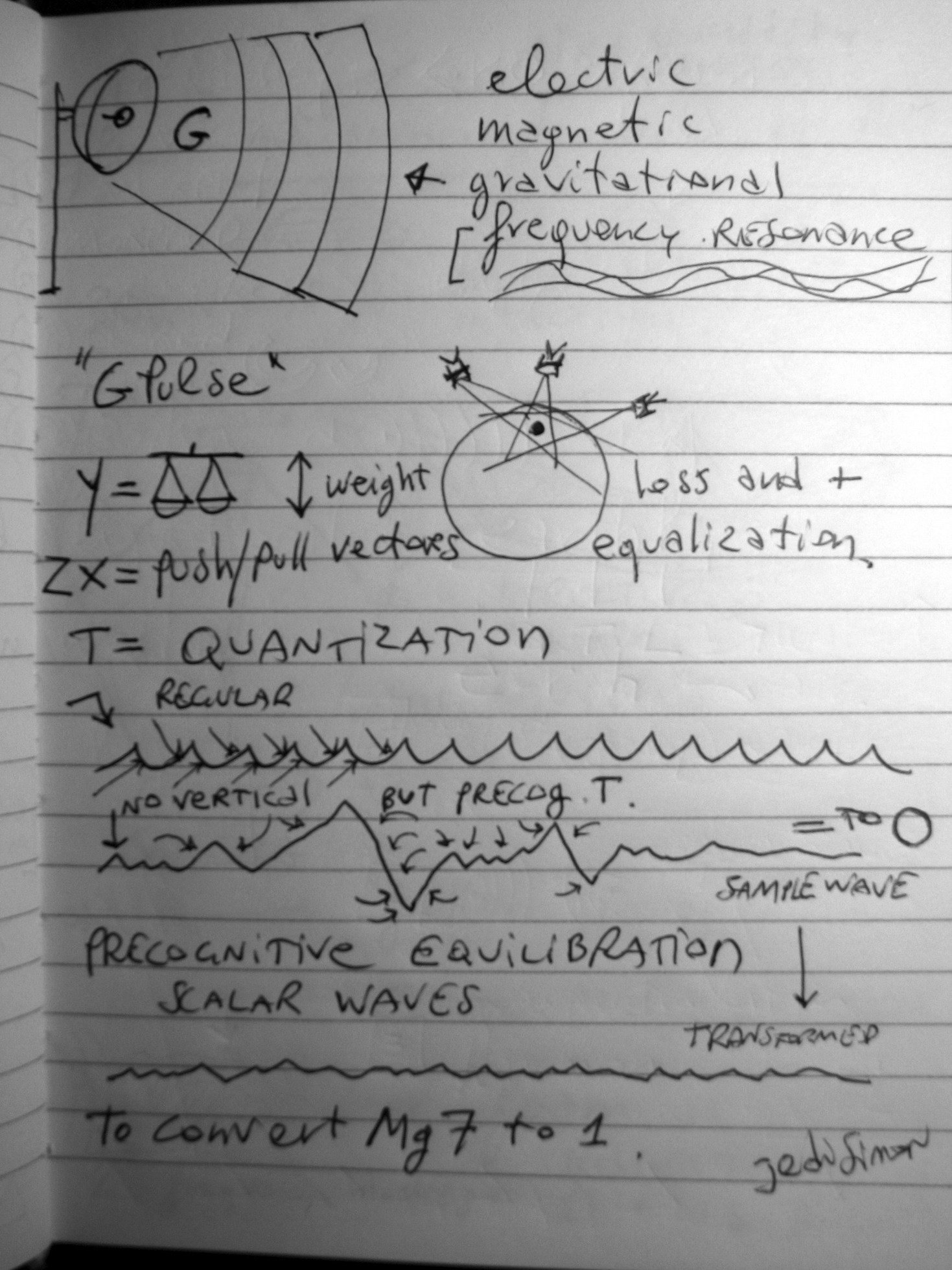
page 5 jedi simon
brainstorming
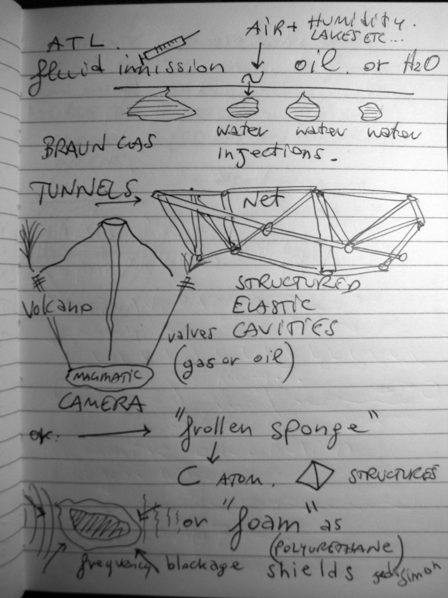
page
6 jedi simon brainstorming
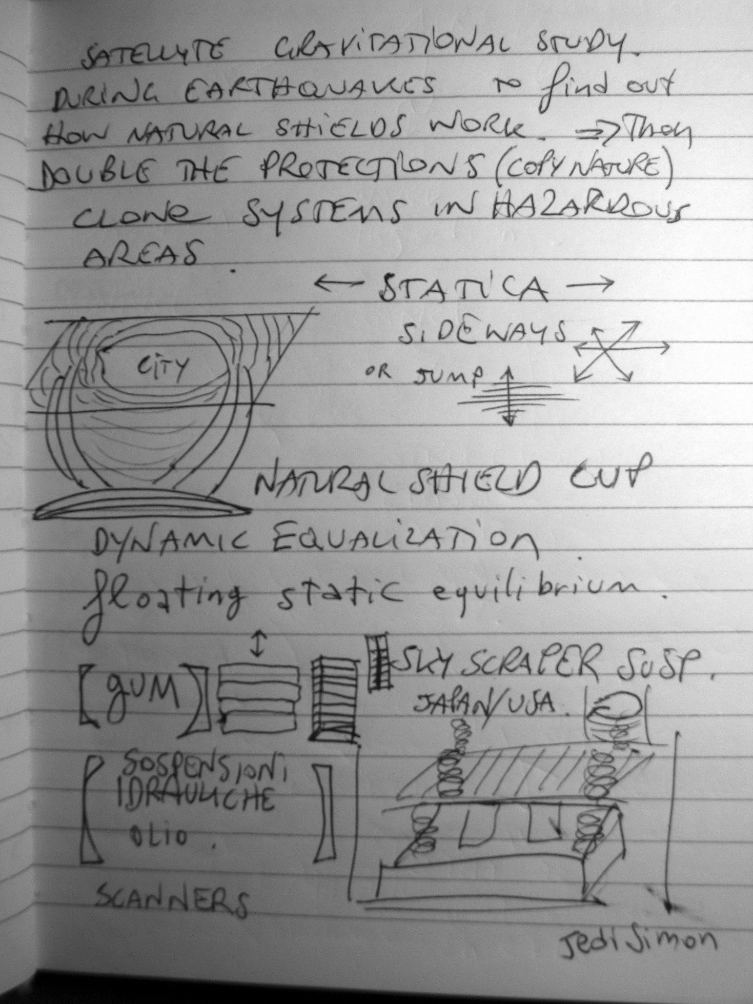
page 8
jedi simon brainstorming
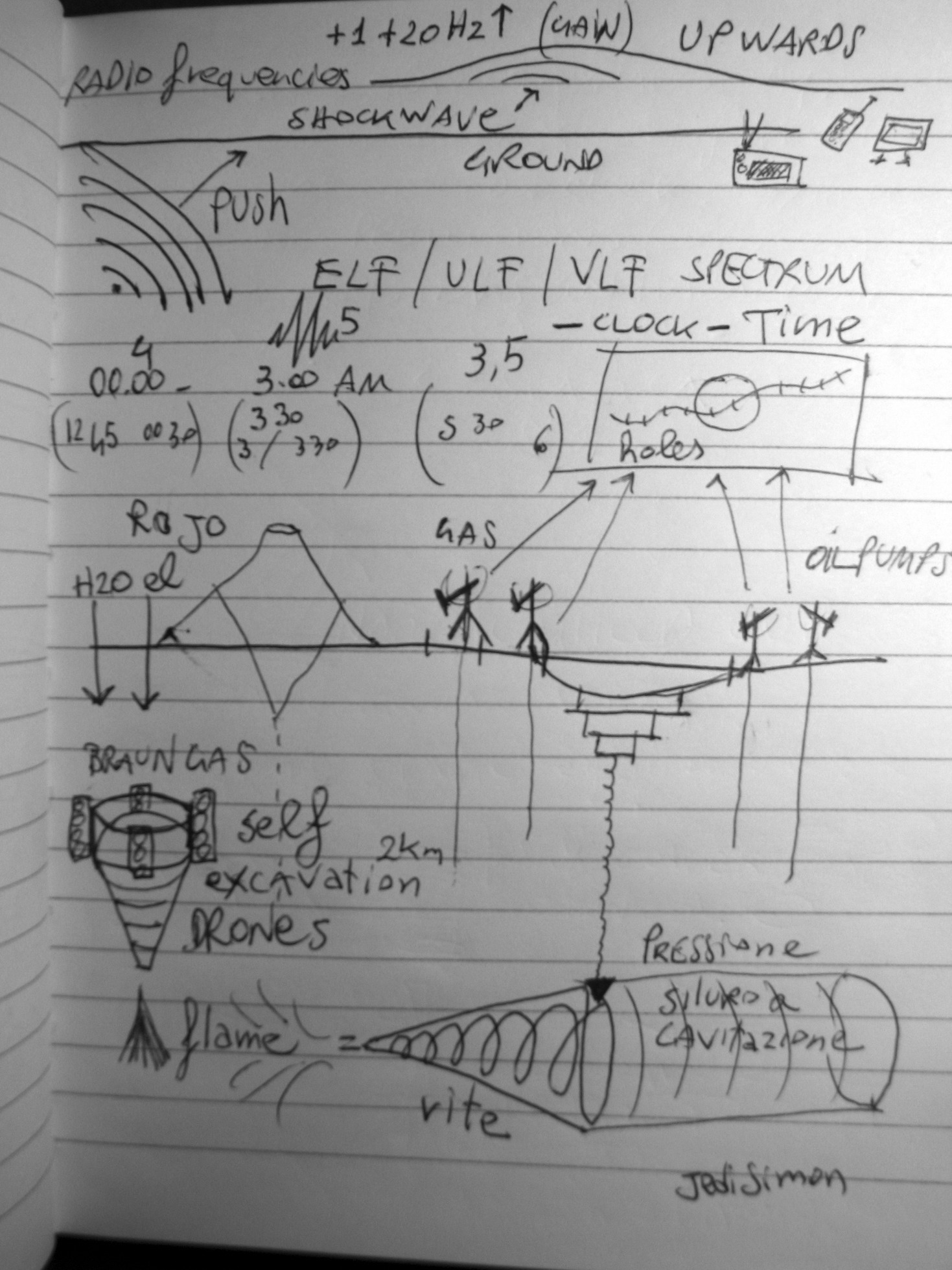
page 9
jedi simon brainstorming
page 9
jedi simon brainstorming
use your heart ... serve life